 2016, Vol. 59


地磁场由95%的主磁场和5%的变化场组成,其中,主磁场由液态地核的磁流体发电机效应和地壳的磁性物质产生,变化场受太阳活动、地球自转、公转等因素影响,变化过程具有时间的连续性(徐文耀,2003).地磁场研究在空间天气预报、地磁导航等领域有着重要应用(徐文耀,2009;袁杨辉,2012).目前,描述全球尺度地磁场的模型有GMM、WMM和CM4等,但这些模型的精度都不高(例如,CM4的时间精度最高为6小时),在局地分析、地磁实时导航等领域不能满足要求(刘代志等,2005;易世华等,2013;牛超等,2014).因此,如何在局部地区获得有效的地磁场分析数据,成为关键技术之一(赵明等,1997;郭才发等,2011).
空间相关的插值方法有Kriging(Goldenberg,2006;张晓明和赵剡,2009; Huang et al.,2012)、多项式插值(孙涵等,2010)、最近邻等,已较多地应用于地磁场的建模分析中.然而,地磁台站信号记录的地磁信号,为时间序列,地磁场数据在时间上具有连续性(李夕海等,2009;曾小牛,2011;曾小牛,2014).以上方法只关注台站空间位置对插值的影响,而忽略了时间域的信息.
时空Kriging方法对Kriging进行了时空域扩展,从而充分利用数据中的时间域信息来进行插值.目前,时空Kriging方法已经在空气质量检测(De Iaco et al.,2003; Nunes and Soares,2005)、雨水建模(李莎等,2011; li et al.,2011; Tang,2002)、风力数据插值(Gneiting,2002)以及地下水建模(Snepvangers et al.,2003; Jost et al.,2005; Cichota et al.,2006; Lark et al.,2006)等领域得到了广泛应用.Gething等(2007)甚至用时空Kriging来分析疟疾门诊病人的数据,将时空Kriging应用到社科数据的分析当中,并取得了良好效果.然而,在地磁学领域,时空Kriging方法至今没有应用,使得插值过程中时间域信息被忽视.
笔者曾研究过用时空Kriging方法来分析地磁场数据所涉及的精度问题、插值过程中数据库容量的选择等.本文重点讨论从空间维度向时间-空间维度扩展过程中,Kriging方法自身发生的变化.在时空变差函数的拟合过程中,将角度信息添加到向量距离的定义当中,提出了改进的时空Kriging算法,并对向量距离中角度信息的权重选择进行讨论.
2 时空Kriging算法及其改进时空Kriging的核心思想,是由Kriging方法在空间域插值的基础上,向时间-空间域进行扩展.
2.1 普通KrigingKriging 方法是以南非矿业工程师D.G.Krige(克里金)名字命名的一项实用空间估计技术,是地质统计学的重要组成部分(Cressie,1988; Bajat et al.,2013).假设在待估计点x的临域内共有n个实测点,即x1,x2,…xn,其样本值为Z(xi).普通Kriging的插值公式为(Cressie,1990; Du and Yang,2012)
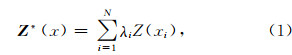
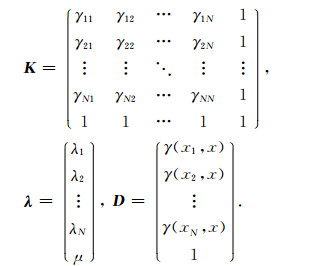
其中的权重系数λi通过Kriging 方程组解算,公式为
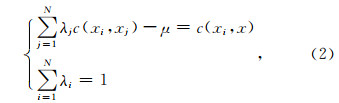
定义变差函数为

由于

式(2)可以转化为
写成矩阵形式为
时空Kriging是在Kriging算法的基础上,引入时间域的连续性与相关性(Rouhani and Myers,1990).用A=(si,tj)示时空域中某一点的坐标,则该点处特征量的值可以表示为邻域内所有点的加权和,即
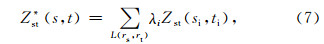

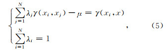
则可以通过Kriging方程组
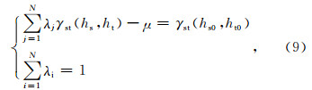
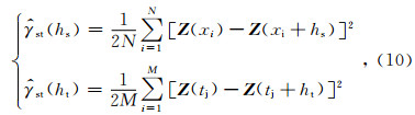
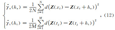
来表示时空域的变差函数(Cressie and Huang,1999),公式为

将式(11)带入到式(9)中,即可解得时空域Kriging方程组.
2.3 改进时空Kriging算法随着定义范围的不同,式(3)中Z(x)与式(10)中Z(x)的含义也发生了变化.如图 1所示,式(3)中Z(x)表示空间中点(x)处地磁场的值,而式(10)中Z(x)则表示,点(x)处各时间采样点所组成的序列.
 | 图 1 Kriging时空扩展演示图 Fig. 1 Illustration of expiation of Spatial Temporal Kriging |
换言之,Z(x)表示对应的空间切片,即Z(x)=(Z(x,t1),Z(x,t2),…,Z(x,tn)),Z(x)亦表示对应的时间切片,即Z(t)=(Z(x1,t),Z(x2,t),…,Z(xm,t)).Z(x)和Z(t)实质上是由切片上各点的值组成的向量,因此,式(10)也可表示为
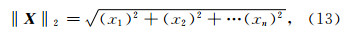
L2范数的定义为
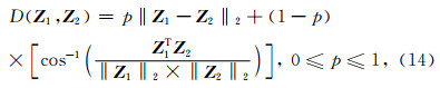
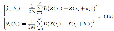
将式(14)代入式(12),得到新向量距离定义下的条件变差函数为
进而构造出时空域联合变差函数γst(hs,ht).
3 实验3.1 数据实验采用的数据,是中国地磁台网及其他几个单独台站(共32个观测台站)从Jan. 1st 2004到Sep.30th2004的地磁场日均值序列.台站位置如图 2所示,五角星分别表示32个观测台站的地理位置,覆盖了经度87.2°E—126.6°E,纬度19.0°N—49.6°N的范围.实验过程中,取式(14)中p=0.3,其理由将在4.2节中作详细讨论和说明.
 | 图 2 台站分布图 Fig. 2 Illustration of monitoring stations |
地磁场的记录数据中,含有一些季节性的积累误差,在插值之前,应该首先对这些成分进行拟合、消除.Kriging与时空Kriging方法都需要满足二次平稳假设,因此,首先对每一个台站的时间序列进行正规化,以使数据独立不相关.
预处理分为两步:
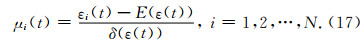
(1)消除数据中的趋势项.各台站的积累误差都不相同,对各台站分别进行拟合,得到趋势项,再进行消除,从而得到余项εi(t)为

(2)用各自的均值、方差对余项εi(t)进行正规化,公式为
预处理的结果如图 3所示,分别以满洲里地磁台(117.4°E,49.6°N)和银川地磁台(106.8°E,38.3°N)数据为例进行说明.图 3a和图 3c中,数据的趋势项可以通过3次多项式进行拟合.对拟合的余项进行正规化,结果如图 3b和图 3d.
 |
图 3 地磁场数据的预处理 (a) (b) 为满洲里地磁台MZL的预处理过程; (c) (d)为银川地磁台YCB的预处理过程. (a) (c)为原始数据及拟合的趋势项; (b) (d)为拟合余项及其正规化结果. Fig. 3 Preprocessing of geomagnetic field data (a) (b) illustrate the preprocessing of data set in monitoring station MZL, while (c) (d) illustrate the station YCB. (a) (c) are the original data and its fitted value, and (b) (d) are residual and its standardized data. |
预处理前后数据的自相关函数如图 4所示.自相关函数是平稳的重要判据之一(李莎等,2012).在预处理之后,自相关函数在非零点处能够迅速地减小,且速度远大于原始数据.由此可见,预处理后数据的平稳性增加,使得数据能更好地满足时空Kriging的二次平稳条件.
 | 图 4 (a)满洲里地磁台MZL和(b)银川地磁台YCB数据的自相函数图 Fig. 4 Autocorrelogram of data sets in monitoring stations (a) MZL and (b) YCB |
时空变差函数的构建,是整个工作的核心.变差函数类型的选择以及拟合的精度,都会影响到时空Kriging插值的精度.根据式(10)和式(15)分别拟合两种距离定义下的条件变差函数.通常用到的变差函数有sphere,index,Gauss,power等,根据观测值的分布情况选择合适的函数进行拟合(De Iaco et al.,2003;李莎等,2012).根据采样数据的形状,试验中空间变差函数均采用sphere函数,时间变差函数采用Gauss函数进行拟合,如图 5所示.从图中对比可以看出,图 5d中观测值比图 5c中更加规则,使得拟合时估计值能够更好地跟踪到观测值,拟合更准确.
 |
图 5 变差函数拟合结果 (a)(b)为空间变差函数拟合,(c)(d)为时间变差函数拟合.(a)(c)是时空Kriging的拟合,(b)(d)是改进后时空Kriging的 拟合结果.(d)中观测值分布平稳,能够较好地集中在拟合曲线周围. Fig. 5 Illustration of fitted variogram functions (a)(b) depict the fitting of space conditional variogram. (c)(d) illustrate the fitting of time conditional variogram. (a)(c) are the results of Spatial Temporal Kriging while (b)(d) is of the improved one. In (d), distribution of sampled data is more stable, and concentrated near the fitted curve. |
本文采用Product-Sum模型,利用条件分布函数来构建时空域变差函数.其模型公式为


 (李莎等,2011).其中参数nugget、sill、range已通过3.3.1 中过程,拟合得到.将取得的时空变差函数分别代入式(10)中,可以解得Kriging方程组,进而算出时空域中任意点的地磁场值.
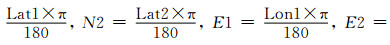
在时空Kriging方法中,取数据库长度为20天.当计算某一个时间点t处的值时,时间区间[t-20,t-1]内的所有观测值都纳入数据库.在87.2°E—126.6°E,19.0°N—49.6°N的范围,取间隔1°进行插值.若地理坐标为A(Lon1,Lat1)和B(Lon2,Lat2),两点间地理距离为


用不同方法插值,并用最近邻法(Barber et al.,1996)和双调和样条插值(Sandwell,1987)做对比试验,结果如图 6所示,依次为最近邻、双调和样条、普通Kriging、时空Kriging、改进时空Kriging插值所得的地磁图.从结果可以看出,图 6a中最近邻方法的分块效应明显,其他方法更为平滑;图 6b中双调和样条方法结果出现了沿纬度方向的条带,而忽视了地磁场在经度方向的差异;图 6c中Kriging方法已可以较好地反映地磁场的分布,准确性优于前二者;通过图 6c和图 6d的对比可以看出,图的左上角处,后者纹理更细致、分辨率更高,时空Kriging在处理插值中常见的边界问题时,效果优于普通Kriging;图 6d与图 6e直观效果差异不大.
 |
图 6 不同方法插值得到的地磁图 (a) 最近邻; (b) 双调和样条; (c) Kriging; (d) 时空Kriging; (e) 改进的时空Kriging. Fig. 6 Interpolation image of different methods (a) Nearest; (b) Double harmonic spline; (c) Kriging; (d) Spatial Temporal Kriging; (e) Improved Spatial Temporal Kriging. |
采用交叉验证中的“留一法”进行实验,即每次假设32个台站中的某一个台站i为未知点(Knotters et al.,1995; Laurenceau and Sagaut,2008),用其他31个台站的值来计算i处地磁场的值  ,并记录它与实测值之间的误差
  ;每个台站作一次未知点,i=1:32为一轮.评价标准为,预测值与实测值之间的平均绝对误差为(Mean Absolute Error,MAE)
均方差为(Mean Square Error,MSE)

时间序列长度为274天,计算时取某一天t的前20天[t-20.t-1]实测值作为时空Kriging的数据库.对[21,274]区间内的每一天,分别用上述5种方法进行插值的交叉验证,结果如图 7所示.不论MAE或MSE,最近邻、双调和样条和Kriging的误差都大于时空Kriging和改进的时空Kriging.而改进的时空Kriging比时空Kriging结果更稳定,误差变化幅度小,MAE集中在1左右,MSE集中在[0,5]的范围内.
 | 图 7 每个时间点处的交叉验证误差 Fig. 7 Statistics of cross validation at each time |
对图 7中各个时刻的MAE和MSE,沿时间轴对误差进行统计分析,其结果如表 1所示.在引入了时间域的信息之后,时空Kriging比之前的空间域传统插值方法,误差减小.但时空Kriging误差的方差比普通Kriging略有增加,反映出误差的波动较大.这种现象在经过改进之后得到解决,改进后时空Kriging误差的各项统计量均达到最小,插值的精度、稳定性明显提高.
| | 表 1 时间域的统计分析 Table 1 Statistics in time domain |
式(14)中,权重p决定了角度信息在向量距离中的比重,进而影响到变差函数拟合的精度.取间隔0.05,在0≤p≤1的范围内考察权重对拟合、插值的影响,结果如图 8所示.当p=0时,向量距离中只有角度信息,幅值信息的缺乏导致大的误差.之后,误差随p的增大而减小;p=0.3时,插值误差达到最小,此时,Mean of MAEs=0.976177666,Mean of MSEs=1.961507859;之后,误差随p增大而增大,p=1时,角度信息缺失,此时向量距离退化为欧式距离,插值结果与时空Kriging相同.在p=0.3处,幅值信息与角度信息达到平衡,使得时间切片间和空间切片间的差异在向量距离中有合适的表达,从而提高变差函数拟合与时空Kriging插值的精度.因此,在本文的实验中,均采用p=0.3.
 | 图 8 权重p对时空Kriging的影响 Fig. 8 Choose of weight p in Improved Spatial Temporal Kriging |
对Kriging方法进行时间-空间域的扩展,其核心是对其变差函数进行时间-空间域的扩展.在加入了时间域信息之后,时空Kriging方法的交叉验证误差减小,插值精度提高;在Kriging变差函数的时空域扩展过程中,将角度信息引入向量距离,从而提出了改进的时空Kriging算法.实验结果表明,新的向量距离能够更有效地表征数据,改进的时空Kriging方法插值精度进一步得到提高.
致谢 文中用到了中国地磁台网等32个地磁台站的地磁场数据,在此一并表示感谢.| [1] | Astola J, Haavisto J, Neuvo Y. 1990. Vector median filters. Proceedings of the IEEE, 78(4): 678-689. |
| [2] | Bajat B, Pejović M, Luković J, et al. 2013. Mapping average annual precipitation in Serbia (1961—1990) by using regression kriging. Theoretical and Applied Climatology, 112(1-2): 1-13. |
| [3] | Barber C B, Dobkin D P, Huhdanpaa H T. 1996. The quickhull algorithm for convex hulls. ACM Transactions on Mathematical Software, 22(4): 469-483. |
| [4] | Cichota R, Hurtado A L B, de Jong van Lier Q. 2006. Spatio-temporal variability of soil water tension in a tropical soil in Brazil. Geoderma, 133(3-4): 231-243. |
| [5] | Cressie N. 1988. Spatial prediction and ordinary kriging. Mathematical Geology, 20(4): 405-421. |
| [6] | Cressie N. 1990. The origins of kriging. Mathematical Geology, 22(3): 239-252. |
| [7] | Cressie N, Huang H C. 1999. Classes of nonseparable, spatio-temporal stationary covariance functions. Journal of the American Statistical Association, 94(448): 1330-1339. |
| [8] | Davis B M, Borgman L E. 1982. A note on the asymptotic distribution of the sample variogram. Mathematical Geology, 14(2): 189-193. |
| [9] | De Iaco S, Myers D E, Posa D. 2002. Nonseparable space-time covariance models: some parametric families. Mathematical Geology, 34(1): 23-42. |
| [10] | De Iaco S, Myers D E, Posa D. 2003. The linear coregionalization model and the product-sum space-time variogram. Mathematical Geology, 35(1): 25-38. |
| [11] | Du R Q, Yang J. 2012. Application of ordinary kriging method in data processing of magnetic survey.//Proceedings of the 2012 7th International Conference on Computer Science & Education. Melbourne, Australia: IEEE, 771-774. |
| [12] | Gething P W, Akinson P M, Noor A M, et al. 2007. A local space-time kriging approach applied to a national outpatient malaria data set. Computers & Geosciences, 33(10): 1337-1350. |
| [13] | Gneiting T. 2002. Nonseparable, stationary covariance functions for space-time data. Journal of the American Statistical Association, 97(458): 590-600. |
| [14] | Goldenberg F. 2006. Geomagnetic navigation beyond the magnetic compass.//Proceedings of the 2006 IEEE/ION Position, Location, and Navigation Symposium. Coronado, CA: IEEE, 684-694. |
| [15] | Guo C F, Zhang L J, Cai H. 2011. Analysis of geomagnetic navigation accuracy under magnetic storms. Chin. J. Space Sci. (in Chinese), 31(3): 372-377. |
| [16] | Huang H, Liu Q, Wang J, et al. 2012. Kriging-based study on the visualization of magnetic method data.//Proceedings of the 2012 International Conference on Image Analysis and Signal Processing. Hangzhou, China: IEEE, 1-6. |
| [17] | Jost G, Heuvelink G B M, Papritz A. 2005. Analysing the space-time distribution of soil water storage of a forest ecosystem using spatio-temporal kriging. Geoderma, 128(3-4): 258-273. |
| [18] | Journel A G. 1986. Geostatistics: Models and tools for the earth sciences. Mathematical Geology, 18(1): 119-140. |
| [19] | Knotters M, Brus D J, Oude Voshaar J H. 1995. A comparison of kriging, co-kriging and kriging combined with regression for spatial interpolation of horizon depth with censored observations. Geoderma, 67(3-4): 227-246. |
| [20] | Lark R M, Bellamy P H, Rawlins B G. 2006. Spatio-temporal variability of some metal concentrations in the soil of eastern England, and implications for soil monitoring. Geoderma, 133(3-4): 363-379. |
| [21] | Laurenceau J, Sagaut P. 2008. Building efficient response surfaces of aerodynamic functions with kriging and cokriging. AIAA Journal, 46(2): 498-507. |
| [22] | Li S, Shu H, Dong L. 2011. Research and realization of Kriging interpolation based on spatial-temporal variogram. Computer Engineering and Applications (in Chinese), 47(23): 25-26. |
| [23] | Li S, Shu H, Xu Z. 2012. Interpolation of temperature based on spatial-temporal kriging. Geomatics and Information Science of Wuhan University (in Chinese), 37(2): 237-241. |
| [24] | Li X H, Liu G, Liu D Z, et al. 2009. Discrimination of nuclear explosions and earthquakes using the nearest support vector feature line fusion classification algorithm. Chinese J. Geophys. (in Chinese), 52(7): 1816-1824, doi: 10.3969/j.issn.0001-5733.2009.07.016. |
| [25] | Liu D Z, Wang R M, Li X H, et al. 2005. Onset point identification of single-channel seismic signal based on wavelet packet and the AR model. Chinese J. Geophys.(in Chinese), 48(5): 1098-1102. |
| [26] | Niu C, Liu D Z, Li X H, et al. 2014. Feature analysis of geomagnetic variation time series based on complexity theory. Chinese J. Geophys. (in Chinese), 57(8): 2713-2723, doi: 10.6038/cjg20140829. |
| [27] | Nunes C, Soares A. 2005. Geostatistical space-time simulation model for air quality prediction. Environmetrics, 16(4): 393-404. |
| [28] | Porcu E, Mateu J, Saura F. 2008. New classes of covariance and spectral density functions for spatio-temporal modelling. Stoch. Environ. Res. Risk Assess., 22(S1): 65-79. |
| [29] | Rouhani S, Myers D E. 1990. Problems in space-time kriging of geohydrological data. Mathematical Geology, 22(5): 611-623. |
| [30] | Sandwell D T. 1987. Biharmonic spline interpolation of GEOS-3 and SEASAT altimeter data. Geophysical Research Letters, 14(2): 139-142. |
| [31] | Snepvangers J J J C, Heuvelink G B M, Huisman J A. 2003. Soil water content interpolation using spatio-temporal kriging with external drift. Geoderma, 112(3-4): 253-271. |
| [32] | Song Y. 2013. Construction and application of the spatio-temporal variability function of groundwater regionalized variable[Master thesis] (in Chinese). Beijing: Beijing Forestry University. |
| [33] | Song Y, Zhang Z, Zhang H X. 2013a. The simulation parameter interpolation of spatial and temporal variability of groundwater. Journal of Arid Land Resources and Environment (in Chinese), 27(8): 120-124. |
| [34] | Song Y, Zhang Z, Zhang H X, et al. 2013b. Evaluation of the spatial and temporal variability of environmental chloride ion in groundwater by simulation. Chinese Journal of Underground Space and Engineering (in Chinese), 9(2): 457-461. |
| [35] | Sun H, Feng Y, An Z Z, et al. 2010. Analysis of variation in geomagnetic field of Chinese mainland based on comprehensive model CM4. Acta Physica Sinica (in Chinese), 59(12): 8941-8953. |
| [36] | Tang Y B. 2002. Comparison of semivariogram models for Kriging monthly rainfall in eastern China. Journal of Zhejiang University Science, 3(5): 584-590. |
| [37] | Trahanias P E, Karakos D G, Venetsanopoulos A N. 1996. Directional processing of color images: theory and experimental results. IEEE Transactions on Image Processing, 5(6): 868-880. |
| [38] | Wang J M, Zhang J, Deng Z B, et al. 2014. Slope deformation analyses with space-time Kriging interpolation method. Journal of China Coal Society (in Chinese), 39(5): 874-879. |
| [39] | Xu A P, Hu L, Shu H. 2011. Extension and implementation from spatial-only to spatiotemporal Kriging interpolation. Journal of Computer Applications (in Chinese), 31(1): 273-276. |
| [40] | Xu W Y. 2003. Geomagnetism (in Chinese). Beijing: Seismological Press. |
| [41] | Xu W Y. 2009. Physics of Electromagnetic Phenomena of the Earth (in Chinese). Hefei: University of Science and Technology of China Press. |
| [42] | Yi S H, Liu D Z, He Y L, et al. 2013. Modeling and forecasting of the variable geomagnetic field by support vector machine. Chinese J. Geophys. (in Chinese), 56(1): 127-135, doi: 10.6038/cjg20130113. |
| [43] | Yuan Y H. 2012. The research of the geomagnetic variation field in the geomagnetic navigation[Ph. D thesis] (in Chinese). Wuhan: Huazhong University of Science and Technology. |
| [44] | Zeng X N, Li X H, Liu D Z, et al. 2011. Regularization analysis of integral iteration method and the choice of its optimal step-length. Chinese J. Geophys. (in Chinese), 54(11): 2943-2950, doi: 10.3969/j.issn.0001-5733.2011.11.024. |
| [45] | Zeng X N, Liu D Z, Li X H, et al. 2014. An Improved iterative Wiener filter for downward continuation of potential fields. Chinese J. Geophys. (in Chinese), 57(6): 1958-1967, doi: 10.6038/cjg20140626. |
| [46] | Zhang Q Y, Wu J T. 2015. Image super-resolution using windowed ordinary Kriging interpolation. Optics Communications, 336: 140-145. |
| [47] | Zhang X M, Zhao Y. 2009. Local geomagnetic field mapping based on kriging interpolation method. Electronic Measurement Technology (in Chinese), 32(4): 122-125. |
| [48] | Zhao M, Zeng X P, Lin Y F. 1997. Nonlinear analysis of magnetic storm in March 13, 1989. Observation and Research on Seismological and Geomagnetism (in Chinese), 18(3): 56-60. |
| [49] | 郭才发, 张力军, 蔡洪. 2011. 磁暴期间的地磁导航精度分析. 空间科学学报, 31(3): 372-377. |
| [50] | 李莎, 舒红, 董林. 2011. 基于时空变异函数的Kriging插值及实现. 计算机工程与应用. 47(23): 25-26. |
| [51] | 李莎, 舒红, 徐正全. 2012. 利用时空Kriging进行气温插值研究. 武汉大学学报. 信息科学版.37(2): 237-241. |
| [52] | 李夕海, 刘刚, 刘代志等. 2009. 基于最近邻支撑向量特征线融合算法的核爆地震识别. 地球物理学报, 52(7): 1816-1824, doi: 10.3969/j.issn.0001-5733.2009.07.016. |
| [53] | 刘代志, 王仁明, 李夕海等. 2005. 基于小波包分解及AR模型的单通道地震波信号初至点检测. 地球物理学报, 48(5): 1098-1102. |
| [54] | 牛超, 刘代志, 李夕海等. 2014. 基于复杂度理论的地磁变化场时间序列特征分析. 地球物理学报, 57(8): 2713-2723, doi: 10.6038/cjg20140829. |
| [55] | 宋莹. 2013. 地下水区域化变量时空变异函数构建及其应用研究[硕士论文]. 北京: 北京林业大学. |
| [56] | 孙涵, 冯彦, 安振昌等. 2010. 利用地磁场综合模型CM4分析中国大陆地区地磁场变化. 物理学报, 59(12): 8941-8953. |
| [57] | 王建民, 张锦, 邓增兵等. 2014. 时空Kriging插值在边坡变形监测中的应用. 煤炭学报, 39(5): 874-879. |
| [58] | 徐爱萍, 胡力, 舒红. 2011. 空间克里金插值的时空扩展与实现. 计算机应用, 31(1): 273-276. |
| [59] | 徐文耀. 2003. 地磁学. 北京: 地震出版社. |
| [60] | 徐文耀. 2009. 地球电磁现象物理学. 合肥: 中国科学技术大学出版社. |
| [61] | 易世华, 刘代志, 何元磊等. 2013. 变化地磁场预测的支持向量机建模. 地球物理学报, 56(1): 127-135, doi: 10.6038/cjg20130113. |
| [62] | 袁杨辉. 2012. 地磁导航中地磁变化场的研究[博士论文]. 武汉: 华中科技大学. |
| [63] | 曾小牛, 李夕海, 刘代志等. 2011. 积分迭代法的正则性分析及其最优步长的选择. 地球物理学报, 54(11): 2943-2950, doi: 10.3969/j.issn.0001-5733.2011.11.024. |
| [64] | 曾小牛, 刘代志, 李夕海等. 2014. 位场向下延拓的改进迭代维纳滤波法. 地球物理学报, 57(6): 1958-1967, doi: 10.6038/cjg20140626. |
| [65] | 张晓明, 赵剡. 2009. 基于克里金插值的局部地磁图的构建. 电子测量技术, 32(4): 122-125. |
| [66] | 赵明, 曾小苹, 林云芳. 1997. 对1989年3月13日磁暴的非线性分析. 地震地磁观测与研究, 18(3): 56-60. |