 2016, Vol. 59


2. 武汉大学地球空间环境与大地测量教育部重点实验室, 武汉 430079;
3. 武汉大学测绘遥感信息工程国家重点实验室, 武汉 430079;
4. 广东工业大学测绘工程系, 广州 510006
2. Key Laboratory of Geospace Environment and Geodesy, Ministry of Education, Wuhan University, Wuhan 430079, China;
3. State Key Laboratory of Information Engineering in Surveying, Mapping and Remote Sensing, Wuhan University, Wuhan 430079, China;
4. Department of Surveying and Mapping, Guangdong University of Technology, Guangzhou 510006, China
重力场精化始终是大地测量学的主要科学目标之一.近年来,随着科技的进步,地球重力场测量手段也越来越丰富,这些观测手段包括传统的地面和船载重力测量、卫星重力测量、航空重力测量、卫星测高.不同的观测手段所获取的重力场信息在时空分布、精度水平、频谱范围上有所差异,这为多尺度、高精度、高分辨率的全球以及局部重力场建模提供了可能.如何融合多源重力场数据确定高精度、高分辨率的重力场模型是当前国际上的研究热点以及前沿问题.
传统的局部重力场逼近主要依托于Stokes/Molodensky边值理论,主要方法包括Stokes/Hotine数值积分法(宁津生等,2003; Ellmann,2005; 束蝉方等,2011; Yildiz et al.,2012)以及最小二乘配置法(Hwang and Hsu,2008; 翟振和和孙中苗,2009; Gilardoni et al.,2013).数值积分法的主要局限在于难于融合多源重力场信息,而最小二乘配置的难点在于如何确定适应多源重力数据的方差-协方差函数及其计算复杂度.径向基函数(radial basis functions)在空间域和频率域都有较好的局部化特性,可以融合多源重力场数据,被广泛地应用到全球以及局部的重力场建模之中.国内外学 者研究了不同类型的径向基函数在局部重力场模型 中的应用,包括:点质量模型(Reilly and Herbrechtsmeier,1978; Lehmann,1993;吴星等,2009); 球谐样条插值模型(Freeden,1984); 泊松小波函数(Wittwer,2009; Slobbe,2013); Slepian函数(Albertella et al.,1999; Simons and Dahlen,2006; Plattner and Simons,2014)及其他包括Blackman核函数、径向多极函数、Abel-Possion核函数在内的基函数(Bentel et al.,2013a,2013b).
基函数的网络设计,包括基函数的深度及其空间分辨率的确定,影响到重力场模型构建的精度水平,国外学者提出了多种方法来确定基函数建模的相关参数.Antunes等(2003)基于点质量模型构建了Lisbon区域的大地水准面模型,通过反复试验确定了该区域点质量模型的网络构建,其构建的大地水准面模型与基于最小二乘配置解算的模型精度相当.Marchenko等(2001)基于陆地重力异常数据利用径向多极函数解算了北欧部分区域的大地水准面模型,利用多极分析法(multipole analysis)确定了多极函数的适宜深度和个数,其大地水准面的精度达到5 cm.Tenzer和Klees(2008)将点质量模型、多极函数、泊松函数及径向小波基函数四种不同的基函数应用于局部重力场建模之中,利用广义交叉检验法(generalized cross validation)确定了不同基函数的适宜深度和个数,基于局部区域实测的陆地重力异常数据建立了该区域的局部重力场模型,结果表明利用不同类型的基函数建立的重力场模型的精度水平相当.Klees等(2008)基于陆地重力异常数据利用泊松小波基函数构建了荷兰区域的似大地水准面模型,并结合广义交叉检验法提出了数据自适应算法用于基函数深度和个数的确定,其构建的重力似大地水准面模型的精度达到1 cm.上述研究表明基函数可用于高精度局部重力场模型的构建,然而现有的研究均基于单一的重力实测数据(主要是陆地重力异常).如何实现融合多源重力观测数据,特别是陆地重力、船载重力、航空重力数据实现陆海统一的区域重力场建模是当前局部重力场建模的热点问题之一,而目前国际上尚无类似成果发表.此外,地形因素影响到局部重力场模型的精度水平,研究地形质量的扰动对于基函数适宜网络设计也是基函数建模的一个关键问题,国内外也未有相关文献对此做细致的分析.
本文以部分欧洲地区的地面重力、船载重力及航空重力数据为基础,研究径向基函数融合多源重力数据构建局部重力场模型的方法.在此基础上,分析地形因素对于径向基函数适宜网络的确定及局部重力场逼近精度的影响.由于泊松小波基函数存在解析形式,在空域中在能量迅速衰减的区域波动较小,且在频域中具有带通特性,适合于局部重力场建模.因此,本文选择泊松小波基函数作为构造基函数实现融合多源重力数据的局部重力场建模.
2 径向基函数的建模方法局部重力场建模归结为对扰动场的研究.基于移去-恢复法,全波段的扰动位信息可表示为:

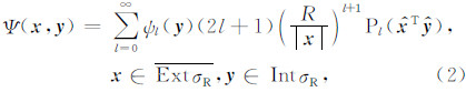
假定σR表示一个完全位于地球内部的球体的 球面,比如Bjerhammar球面.径向基函数可以表示为:
 和
和 分别表示 x 、 y 的单位向量,ψl(y)表示径向基函数的形状因子,决定基函数在空域及频域中的相关特性,d=R- y 也称作基函数的深度.
以泊松小波径向基函数为例,其形状因子可表示为:

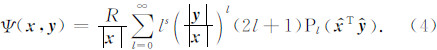
泊松小波径向基函数也存在解析形式,可以通过递推得到任意次的解析核函数,适用于快速计算(Holschneider and Iglewska-Nowak,2007; Tenzer and Klees,2008).
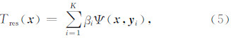
2.2 函数模型及参数估计残余扰动位可表示为有限个泊松小波径向基函数之和:
多源重力场观测数据可表示为扰动位的泛函,本文利用航空重力扰动Δg、陆地及船测重力异常Δg逼近局部重力场,其解算结果以高精度的似大地水准面即高程异常ζ显示.上述重力场的相关参量在球面近似条件下分别与扰动位存在如下函数关系:

结合式(5),对于某一类观测值可以建立观测方程如下:


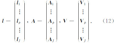
假定不同类型的观测值之间互不相关,观测数据的方差-协方差阵可以表示为:
利用最小二乘原理,基函数的未知参数向量 X 的估值可表示为:
为了对各类观测值进行合理地定权,采用方差分量估计(VCE)的方法,即通过平差随机模型的验 后估计方法重新估计各类观测值的单位权方差因子:

 p2为第p类观测值的验后单位权方差因子,V p= A p
 - l p表示该类观测值的残差,rp表示多余观测数,
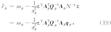
利用(18)式解算多余观测数时需求解并保存法方程N的逆矩阵,对于高分辨率、大区域的局部重力场建模会增加计算复杂度及时间复杂度,本文采用基于随机迹估计的Monte-Carlo方差分量估计(Kusche,2003),其多余观测数可以由(19)式估计:
利用Monte-Carlo方差分量估计对多源观测值定权时需要迭代计算直到每一类观测数据的单位权方差因子都收敛,认为可终止迭代计算,并以本次计算得到的各类观测数据的单位权方差因子定权.本文实际计算中,一般情况下迭代5次可以得到稳定的单位权方差因子估值.
2.3 径向基函数的网络设计基函数的网络设计主要包括两个方面:基函数的三维空间位置以及基函数的个数(空间分辨率).前者又包含两个方面,基函数的平面位置以及深度.对于确定基函数的平面位置,一般而言都是将基函数置于特定的格网点上.Bentel等(2013b)的研究表明利用不同类型的格网确定基函数的平面位置对于局部重力场逼近效果影响较小.参照Klees等(2008)的研究结果,本文选用Fibonacci格网构建基函数的平面位置,计算Fibonacci格网的公式可以参考Eicker(2008).对于基函数深度的确定,通常将基函数置于Bjerhammar球以下的某一球面处(Klees,2008).
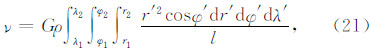
基函数的深度影响到其逼近性质,深度越浅,基函数对高频信号更为敏感;反之,对低频信号更敏感.再者,基函数的深度对解的稳定性、可靠性及精度也存在较大的影响.深度太浅,解的稳定性较高,但可能导致过度拟合的问题,使其可靠性减弱;深度过深,基函数之间的重叠程度增加,导致解的稳定性及精度变差.基函数的个数也会影响到解的稳定性及精度,过多的基函数会引起法方程的病态及过度拟合的问题,过少的基函数导致解的精度偏低.此外,由于地形扰动的影响,不同区域要采用不同的基函数网络建模.在山区,重力场信号与地形起伏存在较强的相关关系,信号波动大,需用较多的浅层基函数建模;在平原区域,地形质量影响较小,信号较为平滑,数量较少的深层基函数就可建立高精度的重力场模型(Slobbe,2013).再者,由于数据分辨率有限,缺乏相应波段的高频重力场信息,忽略地形效应会导致频谱混叠现象,在多山地区可能会导致较大的误差.本文采用残差地形模型(RTM)讨论地形因素对基函数网络设计及局部重力场精度的影响.残差地形模型可逼近地形扰动引起的高频影响,避免频谱混叠效应,在局部重力场建模中有着广泛的应 用(Forsberg and Tscherning,1981; Tziavos et al.,2010; Hirt,2013). 残差地形改正的计算采用基于变密度的球冠体积分(Heck and Seitz,2007),其地形质量引起的扰动位ν可表示为:
基函数的深度及个数的确定可采用广义交叉检验法(GCV)(Klees et al.,2008)以及基于基函数与信号协方差函数拟合的多极分析(Marchenko et al.,2001).广义交叉检验法可能存在难以求取最小值的问题,基于该方法的解可能与最佳参数存在偏差(Hansen and O′Leary,1993).而多极分析方法需对每一个基函数都确定其最佳三维空间位置,增加了算法的时间复杂度.针对上述方法缺点,本文采用最小标准差法(STD)(Slobbe,2013).假设局部区域Ω中共有m个高精度的GPS水准点,利用基函数构建的局部重力场模型可计算第i个GPS水准点上的重力似大地水准面高,记为ζobsi,可视为观测值.而该点实测的几何似大地水准面高,记为ζGPS/levi,可视为真值,两者残差ζresi可表示为:


适当选择不同基函数个数及深度构建一个二维搜索空间,包含不同基函数深度与个数的组合,对于每一种参数组合,利用相应的基函数网络去建立局部重力场模型,通过计算的与实测的似大地水准面高的残差的标准差来评价该模型的精度.其中,精度最高的模型对应的基函数的深度与个数即为最适宜的参数.
3 数值计算与分析 3.1 采用数据基于Eurodem、SRTM(Shuttle Radar Topography Mission)以及GEBCO(General Bathymetric Chart of the Oceans)三种数字地形模型构建了整个欧洲区域高精度、高分辨率(2″×2″)、陆海统一的数字地形模型.全球重力场模型采用代尔夫特理工大学基于GRACE/GOCE联合解算的DGM1S模型,其展开阶数为250阶(Hashemi et al.,2013).收集了整个荷兰、比利时、英国,以及部分德国、法国、丹麦、挪威区域的陆地重力异常数据;部分北海的船载重力异常数据和挪威北部近海区域的航空重力扰动数据.通过交叉点平差的方法完成了对于船载、航空数据中系统偏差的校正;利用阈值法和Hampel滤波完成了多源重力数据的粗差剔除;并利用低通滤波削弱了多源数据中存在的高频噪声的影响.将各类观测数据归算到同一参考框架(ETRS89)及垂直基准(EVRF2007).同时收集了上述国家部分区域的高精度的GPS水准数据,完成了数据预处理工作.
3.2 残差地形改正利用残差地形模型计算多源重力数据的残差地形改正,残余重力观测值如图 1所示.其中,图 1a和1b表示残余陆地重力异常,图 1c和1d表示残余船载重力异常,图 1e和1f表示残余航空重力扰动;图 1a、图 1c及1e表示从原始重力观测值中仅移去全球重力场模型分量后得到的残余重力参量;而图 1b、1d及1f表示移去了全球重力场模型分量以及残差地形改正影响后得到的残余重力参量.结合表 1可知,移去残差地形模型的影响后,残余重力场均有不同程度的平滑.特别是在英国北部、挪威南部及法国、德国的多山地区,其平滑效应尤为明显.就陆地残余重力异常而言,移去残差重力改正后,其标准差从15.924 mGal减少至10.652 mGal,其平滑程度改善了约33%.对残余船载重力异常而言,移去残差地形影响后,其标准差从13.994 mGal减为12.403 mGal,改善了约为11%.其平滑程度没有陆地重力数据明显,主要原因为基于GEBCO海洋测深模型构建的海洋数字地形模型的精度及空间分辨率都较低(原始的分辨率为30″×30″),基于残差地形模型的重力场高频信号逼近的精度也会受到影响.在移去航空重力测量中高频信号的影响时发现,其残余重力扰动的标准差仅从10.594 mGal下降到10.446 mGal.一方面受制于海洋数字地形模型的精度及分辨率(航空重力测量位于近海区域),另一方面重力场的高频信号随高度的增加迅速衰减,较之于地面重力测量,航空重力测量对重力场高频信号的敏感度较弱,利用残差地形模型的重力场高频信号逼近的影响也随之减弱.
 | 图 1 残余重力观测数据Fig. 1 Residual gravity observations |
| | 表 1 残余重力数据统计信息 (单位: mGal) Table 1 The statistics of the residual gravity observations (unit: mGal) |
为了研究地形质量对基函数网络设计的影响,分别利用“两步法”和“三步法”构建了局部重力场模型.不同地形区域基函数的适宜网络设计存在差异,研究中分别选择平原及多山区域作为实验区域.平原区域ΩA选为覆盖荷兰、比利时以及部分德国、法国和北海区域,其纬度范围为49°~56°,经度范围为0°~10°.基函数的深度变化范围为30~50 km,变化 步长为5 km;空间分辨率变化范围为7.2~9.0 km,步长为0.3 km.利用该区域部分GPS水准数据确定基函数的最佳网格设计,结果见图 2及表 2和表 3.图 2a、2b分别为“两步法”和“三步法”的检核结果.图 2中灰色格网表示基函数之间重叠程度增加而导致法方程的严重病态问题.结果表明:基于“两步法”和“三步法”构建基函数的网络最佳深度及最适宜的空间分辨率相一致,其深度均为40 km,最适宜的基函数的个数为7394,即空间分辨率约为8.7 km.该区域地形起伏较小,地形质量引入的高频效应对于基函数网格设计影响较小.值得注意的是,较之于 “两步法”,基于“三步法”建立的模型的最佳精度提高了4 mm.
 | 图 2 重力似大地水准面与GPS水准确定的高程异常差距的标准差(区域ΩA)Fig. 2 The std of the differences between the gravimetric quasi-geoid and GPS/leveling-derived height anomaly (ΩA) |
| | 表 2 利用“两步法”基于不同基函数网络解算的局部重力场模型的精度水平(单位:m) Table 2 The accuracy of different quasi-geoids computed by using "two steps" method based on various radial basis functions′ network design (unit:m) |
| | 表 3 利用“三步法”基于不同基函数网络解算的局部重力场模型的精度水平(单位:m) Table 3 The accuracy of different quasi-geoids computed by using "three steps" method based on various radial basis functions′ network design (unit:m) |
多山区域ΩB选为覆盖英国及部分北海的局部地区,其纬度范围为51°~59°,经度范围为-6°~-1°.基函数的深度变化范围为20~50 km,变化步长为5 km;空间分辨率变化范围为7.2~9.2 km,步长为0.2 km.由于该区域缺乏高精度的GPS水准数据,利用欧洲似大地水准面2008模型(EGG08)作为参考模型来检核基于不同基函数网络设计解算的局部重力场模型的精度水平,结果见图 3及表 4和表 5.图 3a、3b分别表示基于“两步法”和“三步法”的结果.可以得出,引入残差地形改正之后,基函数的最佳深度由25 km增加为35 km,而最适宜的基函数个数从14518(空间分辨率约为8.0 km)减少到11894(空间分辨率约为8.6 km).由于该区域地形起伏及复杂程度较大,地形质量对于高频重力场信号的逼近影响较大,移去残差地形改正之后,残余重力场信号频谱向低频方向移动导致最佳构造基变为埋深更深、对低频信号更为敏感的深部基函数.同理,移去残差地形改正之后,由于重力场高频扰动的衰减,残余重力场变化更为缓和,较少的基函数便能高精度地逼近真实局部重力场.同时,较之于“两步法”建立的模型的最佳精度(0.097 m),基于“三步法”建立的局部重力场模型的最佳精度提高了约0.05 m,其精度水平的改善程度约为50%.基于上述分析,在多山区域,利用残差地形模型的方法平滑了局部重力场信号,简化了基函数的网络设计(减少的基函数个数相当于总体基函数18%),提高了局部重力场模型逼近的精度.
 | 图 3 重力似大地水准面与EGG08似大地水准面差距的标准差(区域ΩB)Fig. 3 The std of the differences between the gravimetric quasi-geoid and EGG08 reference model (ΩB) |
| | 表 4 利用“两步法”基于不同基函数网络得到的局部重力场模型的精度水平(单位:m) Table 4 The accuracy of different quasi-geoids computed by using “two steps” method based on various radial basis functions′ network design (unit: m) |
| | 表 5 利用“三步法”基于不同基函数网络得到的局部重力场模型的精度水平(单位:m) Table 5 The accuracy of different quasi-geoids computed by using “three steps” method based on various radial basis functions′ network design (unit: m) |
试算区域Ω包括子区域ΩA及ΩB,其纬度范围为49°~61°,经度范围为-6°~10°.根据上述计算结果,在不同区域分别构造适宜的基函数网络用于局部重力场的逼近.分别采用“两步法”及“三步法”建立局部重力场模型.图 4为两种方法解算的重力观测值残差,图 4a表示“两步法”解算的残差,较大的残差集中在英国、挪威、比利时、法国及德国部分的多山区域,并显示出高频扰动的特性.受实测重力数据分辨率的影响,地形质量带来的高频效应不能完全被径向基函数恢复,在地形起伏较大的区域建立的重力场模型的精度较低.利用“三步法”解算时,移去了地形扰动带来的高频效应,其残余重力场变得更为平滑,模型精度得到显著提升,其高频性质的残差得到大幅度削弱,见图 4b.从表 6可知,移去地形质量的影响之后,陆地重力异常的残差的标准差由4.055 mGal减小到1.453 mGal.
 | 图 4 重力观测值残差Fig. 4 The residuals of the gravity observations |
| | 表 6 重力观测值残差统计信息(单位:mGal) Table 6 The statistics of the residuals of the gravity observations (unit: mGal) |
分别利用位于荷兰、比利时以及覆盖部分德国区域的GPS水准数据评价局部重力场模型的精度水平.基于“三步法”构建的局部重力场模型的检核 结果见图 5(残差中移去了平均值的影响)、表 7.结果表明利用“三步法”构建的局部重力似大地水准面模型在荷兰、比利时及德国相关区域,其精度分别达到1.12 cm、2.80 cm以及2.92 cm.研究还发现重力似大地水准面模型与GPS水准确定的高程异常存在厘米量级的偏差,见表 7.引起这些系统误差 的原因包括:多源重力数据归算处理中未经完全消 除的系统偏差;高程基准转换参数的不准确性引入的系统误差及全球重力场模型带来的系统偏差等因素.未来的工作除了进一步改善数据预处理的方法之外,还需要利用适当的方法联合重力似大地水准 面与GPS水准数据,削弱上述系统误差带来的影响.
 | 图 5 基于模型解算的高程异常和利用GPS/水准计算的高程异常的差异Fig. 5 The difference between the gravimetric height anomalies and GPS/leveling-derived height anomalies |
| | 表 7 局部重力似大地水准面的精度评价(单位:cm) Table 7 The evaluation of the gravimetric quasi-geoid over the regional area (unit: cm) |
研究了基于泊松小波基函数融合多源数据的局部重力场建模方法,利用最小标准差法确定了基函数的适宜网络,分析了地形扰动引起的高频效应对于基函数网络设计及局部重力场建模精度的影响.基于Monte-Carlo方差分量估计的定权方法,融合实测的陆地重力异常、船载重力异常及航空重力扰动数据构建了局部区域陆海统一的似大地水准面模型.主要结论如下:
(1)基函数的网络设计对于局部重力场逼近的精度影响较大,由于地形扰动的影响,不同区域可能需要构建不同的基函数网络.
(2)受制于重力数据分辨率的影响,忽略地形质量带来的高频效应会导致频谱混叠现象,此时利用基函数建立的局部重力场模型缺乏对于高频信息恢复的能力,会影响建立模型的精度水平.利用残差地形模型平滑了局部重力场高频扰动信号,简化了基函数的网络设计,提高了模型精度.平原区域其相应的重力似大地水准面的精度提升了4 mm;多山地区其精度提高了5 cm.
(3)基函数能够融合多源数据精确地逼近局部重力场模型,基于“三步法”构建的局部重力似大地水准面在荷兰、比利时及德国相关区域,其精度分别达到1.12 cm、2.80 cm以及2.92 cm.
(4)由于多源重力数据中未经完全消除的系统偏差、高程基准转换引入的偏差以及全球重力场模型带来的系统误差等因素,使得重力似大地水准面与GPS水准测定的高程异常存在厘米级的系统偏差,需采用适当的方法(如改正曲面法或最小二乘配置法)联合重力似大地水准面与GPS水准数据,削弱上述系统误差带来的影响.
致谢 感谢代尔夫特理工大学Rol and Klees教授提供的相关重力数据及计算软件.感谢两位审稿专家提出的宝贵意见.| [1] | Albertella A, Sansò F, Sneeuw N. 1999. Band-limited functions on a bounded spherical domain:the Slepian problem on the sphere. Journal of Geodesy, 73(9):436-447. |
| [2] | Antunes C, Pail R, Catalão J. 2003. Point mass method applied to the regional gravimetric determination of the geoid. Stud. Geophys. Geod., 47(3):495-509. |
| [3] | Bentel K, Schmidt M, Gerlach C. 2013a. Different radial basis functions and their applicability for regional gravity field representation on the sphere. GEM-International Journal on Geomathematics, 4(1):67-96. |
| [4] | Bentel K, Schmidt M, Rolstad Denby C. 2013b. Artifacts in regional gravity representations with spherical radial basis functions. Journal of Geodetic Science, 3(3):173-187. |
| [5] | Eicker C. 2008. Gravity field refinement by radial basis functions from in-situ satellite data[Ph. D. thesis]. Bonn:Bonn University. |
| [6] | Ellmann A. 2005. Computation of three stochastic modifications of Stokes's formula for regional geoid determination. Computers & Geosciences, 31(6):742-755. |
| [7] | Forsberg R, Tscherning C C. 1981. The use of height data in gravity field approximation by collocation. Journal of Geophysical Research, 86(B9):7843-7854. |
| [8] | Freeden W. 1984. Spherical spline interpolation-basic theory and computational aspects. Journal of Computational and Applied Mathematics, 11(3):367-375. |
| [9] | Gilardoni M, Reguzzoni M, Sampietro D. 2013. A least-squares collocation procedure to merge local geoids with the aid of satellite-only gravity models:the Italian/Swiss geoids case study. Boll. Geof. Teor. Appl., 54(4):303-319. |
| [10] | Hansen P C, O'Leary D P. 1993. The use of the L-curve in the regularization of discrete ill-posed problems. Journal of Scientific Computing, 14(6):1487-1503. |
| [11] | Hashemi F H, Ditmar P, Klees R, et al. 2013. The static gravity field model DGM-1S from GRACE and GOCE data:computation, validation and an analysis of GOCE mission's added value. Journal of Geodesy, 87(9):843-867. |
| [12] | Heck B, Seitz K. 2007. A comparison of the tesseroid, prism and point-mass approaches for mass reductions in gravity field modelling. Journal of Geodesy, 81(2):121-136. |
| [13] | Hirt C. 2013. RTM gravity forward-modeling using topography/bathymetry data to improve high-degree global geopotential models in the coastal zone. Marine Geodesy, 36(2):183-202. |
| [14] | Holschneider M, Iglewska-Nowak I. 2007. Poisson wavelets on the sphere. Journal of Fourier Analysis and Applications, 13(4):405-419. |
| [15] | Hwang C, Hsu H Y. 2008. Shallow-water gravity anomalies from satellite altimetry:Case studies in the east china sea and Taiwan strait. Journal of the Chinese Institute of Engineers, 31(5):841-851. |
| [16] | Klees R, Tenzer R, Prutkin I, et al. 2008. A data-driven approach to local gravity field modelling using spherical radial basis functions. Journal of Geodesy, 82(8):457-471. |
| [17] | Kusche J. 2003. Noise variance estimation and optimal weight determination for GOCE gravity recovery. Advances in Geosciences, 1:81-85. |
| [18] | Lehmann R. 1993. The method of free-positioned point mass-geoid studies on the Gulf of Bothnia. Bulletin Géodésique, 67(1):31-40. |
| [19] | Marchenko A N, Barthelmes F, Meyer U, et al. 2001. Regional Geoid Determination:An Application to Airborne Gravity Data in the Skagerrak. Technical report, Geo-Forschungs Zentrum Potsdam. |
| [20] | Ning J S, Luo Z C, Yang Z J, et al. 2003. Determination of Shenzhen geoid with 1 km resolution and centimeter accuracy. Acta Geodaetica et Cartographica Sinica(in Chinese), 32(2):102-107. |
| [21] | Panet I, Kuroishi Y, Holschneider M. 2011. Wavelet modelling of the gravity field by domain decomposition methods:an example over Japan. Geophysical Journal International, 184(1):203-219. |
| [22] | Plattner A, Simons F J. 2014. Spatiospectral concentration of vector fields on a sphere. Applied and Computational Harmonic Analysis, 36(1):1-22. |
| [23] | Reilly J P, Herbrechtsmeier E H. 1978. A systematic approach to modeling the geopotential with point mass anomalies. Journal of Geophysical Research, 83(B2):841-844. |
| [24] | Shu C F, Li F, Li M F, et al. 2011. Determination of GPS/gravity quasi-geoid using the Bjerhammar method. Chinese J. Geophys.(in Chinese), 54(10):2503-2509, doi:10.3969/j.issn.0001-5733.2011.10.008. |
| [25] | Simons F J, Dahlen F A. 2006. Spherical Slepian functions and the polar gap in geodesy. Geophysical Journal International, 166(3):1039-1061 |
| [26] | Slobbe D C. 2013. Roadmap to a mutually consistent set of offshore vertical reference frames[Ph. D. thesis]. Delft:Delft University of Technology. |
| [27] | Tenzer R, Klees R. 2008. The choice of the spherical radial basis functions in local gravity field modeling. Stud. Geophys. Geod., 52(3):287-304. |
| [28] | Tenzer R, Klees R, Wittwer T. 2012. Local gravity field modelling in rugged terrain using spherical radial basis functions:case study for the Canadian rocky mountains.//Kenyon S, Pacino M C, Marti U eds. Geodesy for Planet Earth. Berlin Heidelberg:Springer-Verlag, 401-409. |
| [29] | Tziavos I N, Vergos G S, Grigoriadis V N. 2010. Investigation of topographic reductions and aliasing effects on gravity and the geoid over Greece based on various digital terrain models. Surveys in Geophysics, 31(1):23-67. |
| [30] | Wittwer T. 2009. Regional gravity field modelling with radial basis functions[Ph. D. thesis]. Delft:Delft University of Technology. |
| [31] | Wu X, Zhang C D, Zhao D M. 2009. Point mass harmonic analysis method based on spherical boundary value problem. Chinese J. Geophys.(in Chinese), 52(12):2993-3000, doi:10.3969/j.issn.0001-5733.2009.12.008. |
| [32] | Yildiz H, Forsberg R, Ågren J, et al. 2012. Comparison of remove-compute-restore and least squares modification of Stokes' formula techniques to quasi-geoid determination over the Auvergne test area. Journal of Geodetic Science, 2(1):53-64. |
| [33] | Zhai Z H, Sun Z M. 2009. Continuation model construction and application analysis of local gravity field based on least square collocation. Chinese J. Geophys.(in Chinese), 52(7):1700-1706, doi:10.3969/j.issn.0001-5733.2009.07.004. |
| [34] | 宁津生, 罗志才, 杨沾吉等. 2003. 深圳市1KM高分辨率厘米级高精度大地水准面的确定. 测绘学报, 32(2):102-107. |
| [35] | 束蝉方, 李斐, 李明峰等. 2011. 应用Bjerhammar方法确定GPS重力似大地水准面. 地球物理学报, 54(10):2503-2509, doi:10.3969/j.issn.0001-5733.2011.10.008. |
| [36] | 吴星, 张传定, 赵东明. 2009. 基于球面边值问题的点质量调和分析方法. 地球物理学报, 52(12):2993-3000, doi:10.3969/j.issn.0001-5733.2009.12.008. |
| [37] | 翟振和, 孙中苗. 2009. 基于配置法的局部重力场延拓模型构建与应用分析. 地球物理学报, 52(7):1700-1706, doi:10.3969/j.issn.0001-5733.2009.07.004. |