地球固态内核在其平衡位置附近的平动振荡是地球自由振荡基本核模，也是基本简正模之一，或称之为Slichter模(Slichter，1961)，包括赤道面上的正向运动、地球自转轴方向上的轴向运动和赤道面上的逆向运动(Slichter，1961; Smith，1976).对于非旋转、球对称、理想弹性和各向同性地球模型(SNREI)，简并的Slichter模是周期最长的一阶球型振荡模态(₁S₁)，它的本征位移为一阶球型位移.与其他的地球自由振荡简正模一样，地球的自转、椭率和3-D结构将会引起Slichter模的谱线分裂，形成一组方位角级数m分别为-1，0和1的三条谱线，分别对应地球固态内核平动振荡的三重分裂谱峰(王迪晋，2012; Ding and Shen，2013; Shen and Ding，2013).Slichter模的本征周期与内核边界(inner core boundary，ICB)处的密度跳跃Δρ_ICB有密切关联(Crossley et al.，1992; Rieutord，2002)，因此Slichter模三重分裂谱线的本征周期观测有利于约束地球内外核边界处的密度跳跃和黏滞度.

研究表明，重力测量可有效应用于探测地球内部构造特征和动力学现象(Melchior and Ducarme，1986).然而地球固体内核平动振荡引起的地表重力变化信号非常微弱，易淹没于Slichter模所在的亚潮汐频段的台站背景噪声中，探测难度很大.研究表明(Smith，1976; Crossley et al.，1991)，大地震激发的Slichter模导致地表重力信号的变化幅度可达 nGal量级，与超导重力仪(superconducting gravimeter，SG)的观测精度(10^-11m·s^-2)相当.SG是目前观测精 度最高、稳定性和连续性最好的地球重力场信号观 测仪器，对重力场变化有很高的灵敏度，在低于0.8 mHz 频段优于当前最好的宽频地震仪；它在低频段具有极低的噪声水平，特别适用于长周期信号的观测，在研究地球自由振荡模态方面优势明显(Hinderer et al.，1995; Rosat et al.，2004，2006).相关学者在利用SG数据检测内核平动振荡方面做了许多有益的尝试，以Smylie为代表的少数科学家基于亚地震波近似的理论计算结果，声称在SG的长期观测资 料的亚潮汐频段(0.172~0.285cph)发现了“Slichter模”弱共振信号(Smylie，1992; Smylie et al.，1993; Courtier et al.，2000)，并在此基础上研究了内核边界附近的密度和黏滞度，但他们的结果受到了很多科学家的质疑(Hinderer et al.，1995; Jensen et al.，1995; Rosat et al.，2003).至今，是否已观测到甚至能否观测到Slichter模三重分裂，争议很大，这也成为当今国际地学界的一个热点研究课题.

用于探测地球简正模态的方法很多，主要将它们分为频率域方法和时间域方法.早期应用于探测简正模态的研究方法主要在频率域，主要包括以下五种方法(Ding and Shen，2013)：(1)最小二乘谱 分析(LSSA，Vaníek，1969)；(2)单线态剥离(SS)法(Gilbert，1971)；(3)积谱分析(PSA，Smylie et al.，1993)；(4)交叉谱分析(Hinderer et al.，1995)；(5)矩阵自回归分析(MARA，Masters et al.，2000).后来逐渐发展到频率域和时间域相结合的方法，主要包括以下四种方法：(1)球谐叠加技术(SHS，Buland et al.，1979)；(2)多台站试验技术(MSE，Courtier et al.，2000)；(3)非线性阻尼谐波分析法(Rosat et al.，2008)；(4)最优序列估计(OSE，Ding and Shen，2013).

EEMD是Wu和Huang(2009)基于噪声辅助数据分析(NADA)理论，对EMD方法(Huang et al.，1998)做出的进一步改进方法，其目的是减弱或消除模态混叠效应(mode mixing effect)及端点效应(end effect)，使分解得到的IMF具有更集中的频率信息，有助于提取数据中的真实信号.应用EEMD处理SG重力残差序列，可有效过滤重力残差中非目标频段的信号，增强目标模态的信噪比，有利于目标微弱信号的提取，其有效性和优越性参见Shen和Ding(2014).基于最小二乘原理的OSE方法是对MSE方法的改进，提供了以更高的信噪比剥离单线态信号的手段，可有效应用于探测Slichter模三重分裂.本文基于全球地球动力学计划(GGP)观测网提供的超导重力仪观测资料，利用EEMD方法提取经常规预处理(包括潮汐改正、气压改正和极移改正)后的重力残差中包含目标频段(0.15~0.30cph)的IMFs作为最终的重力残差；结合OSE和PSA方法探测相应频段内与地球固态内核平动振荡有关的重力信号；最后应用基于Prony方法的频率域自回归估计(AR)方法(Prony，1795; Chao and Gilbert，1980)，估算可能的弱共振信号的中心频率，并结合最小二乘误差传播定律估算其精度.

为探测Slichter模三重分裂信号，本文选取了全球地球动力学计划(GGP)观测网中的9个超导重力仪台站在2004苏门答腊大地震发生5小时后连续13200 h、采样率为1h的观测数据，这些台站分别是德国的Bad Homburg、Moxa、Wettzell，加拿 大的Canberra，奥地利的Vienna，比利时的Membach，意大利的Medicina，南非的Southl and ，日本的Matsushiro，相关信息见表 1.从台站地理位置来看，除美洲和南极洲以外，其他大洲均有台站，排除了台站局部区域分布的影响，在一定程度上保证了探测结果的可靠性.

表 1(Table 1)

表 1 9个超导重力仪台站的相关信息 Table 1 Relevant information of 9 SG stations 台站名称 国际代码 仪器编码 经度/(°) 纬度/(°) 高程/m Bad Homburg BH GWR CD030_L 8.6113 50.2285 190 Canberra CB GWR C031 149.00766 -35.32064 762.749 Medicina MC GWR C023 11.645 44.5219 28 Membach MB GWR C02 6.0066 50.6093 250 Moxa MO CD034_L 50.645 11.616 455 Southland SU GWR D037_L 20.8109 -32.3814 1791 Wettzell WE GWR CD029_L 49.144 12.878 613.7 Vienna VI GWR C025 16.3565 48.2489 192.74 Matsushiro MA GWR T011 138.2032 36.5439 451.1

表 1 9个超导重力仪台站的相关信息 Table 1 Relevant information of 9 SG stations

为减少数据预处理带来的人为影响，所有9个观测序列采用相同的预处理和调和分析方法.其处理过程主要包括以下3个步骤.

(1)利用德国Wenzel 研制的ETERNA标准潮汐分析软件(Wenzel，1996)，精密确定重力潮汐参数(包括振幅因子和相位滞后)，并从各原始观测序列中扣除相应的重力潮汐信号(包括固体潮和海潮负荷效应)；采用国际上通用的大气重力导纳值法，得到气压观测数据与其重力影响之间的对应关系，计算出气压重力影响并实施改正； 根据IERS(International Earth Rotation Service)提供的地球自转参数计算极移效应并加以扣除，得到重力残差序列.

(2)选择0.15~0.30cph频段作为目标频段，将EEMD作为一种并矢滤波器，提取含有目标频段的IMFs作为最终的重力残差.为描述该过程，我们以意大利 Medicina台站重力残差序列为例，对重力残差序列实施EEMD分解，可得到12个IMF和一个残余趋势项(图 1).为详细了解各IMF的频率信息，我们对每个IMF作傅利叶变换得到各自的振幅谱.图 2给出了重力残差经过EEMD分解后得到的前6个IMF的振幅谱.可以看到，按照分解的顺序IMF的能量分别集中在由高到低分布的频段上；在目标频段内，除IMF1和IMF2以外，其他IMF的振幅几乎为零，因此我们选择IMF1+IMF2作为最终的重力残差.图 3给出了EEMD处理前后的重力残差在目标频段的振幅谱，图中黑色曲线表示原始重力残差的振幅谱，红色虚线表示经过EEMD处理后的重力残差振幅谱.可以看出，原始重力残差经EEMD处理后，目标频段的噪声水平并没有比较明 显的降低；尽管Shen and Ding(2014)已验证了EEMD 在探测微弱信号时能相对增强它们的信噪比(SNR)，但对于某些未知频率的弱信号(如Slichter模，我们只能结合前人的理论研究结果确定一个宽泛的目标频段)，EEMD的效果并不明显，但这并不妨碍我们利用EEMD过滤某些残余的潮汐信号.确切地说，EEMD 有助于提高SNR.

图 1

Fig. 1

图 1 Medicina台站长度为13200 h的重力残差序列及其EEMD分解结果，EEMD分解得到12个IMF和1个残余趋势项(纵坐标单位为nm·s-2)Fig. 1 Residual gravity series and EEMD decomposition for 13200 hours at the Medicina station, and 12 IMFs and 1 remainder obtained after using EEMD (The unit of Y-axis is nm·s-2)

图 2

Fig. 2

图 2 Medicina台站重力残差经过EEMD分解后得到的前六个IMF的振幅谱(纵坐标为振幅，单位为nm·s-2)Fig. 2 Amplitude spectra of the first six IMFs of residual gravity series after using EEMD at the Medicina station (Y-axis is the amplitude with unit nm·s-2)

图 3

Fig. 3

图 3 Medicina台站重力残差的振幅谱 黑色实线为没有实施EEMD处理的重力残差振幅谱曲线，红色虚线为EEMD处理后的重力残差振幅谱曲线.Fig. 3 Amplitude spectra of the residual gravity series at the Medicina station Black curve is amplitude spectra without using EEMD, and red dashed curve is amplitude spectra after using EEMD.

(3)将EEMD处理后的各台站最终重力残差序列分为3个无重叠的子数据块S_1i(t)、S_2i(t)、S_3i(t)(i=1、2、…、9)，即每个台站重力残差按照时间段被分成3等份，每份数据长度为4400 h，则可得到27个新的残差序列，供后续使用.

Ding和Shen(2013)基于最小二乘原理，对多台站试验(MSE)技术作了进一步改进，提出了一种时间域的最优序列估计(OSE)方法，主要解决了MSE方法中随机噪声影响问题.MSE方法和OSE方法，二者均是基于目标模态的特性而提出的方法，旨在将多重态自由振荡信号的单线态逐个剥离，达到识别信号的目的(丁浩，申文斌，2013).

任一台站的观测重力残差g_j(t)包含三个平动振荡模信号，分别为赤道面正向、自转轴方向和赤道面逆向振荡(即Slichter模的三个单线态信号)，可 表示为(Courtier et al.，2000; Ding and Shen，2013)

当台站数N>3时，可将式(1)表达为矩阵形式为

考虑到MSE方法的限制，Ding和Shen(2013)采用最小二乘方法来估计未知时间序列a_pe^iω_pt、a_ae^iω_at和a_re^iω_rt，方程(2)的最小二乘解为

采用OSE方法可以剥离出Slichter模的三个单线态信号，且三个独立的时间序列可以表示为

为作比较，我们设计了以下2个方案来处理相同的3个数据块，方案中所有功率谱密度均采用“log”形 式，得到的积谱密度单位相同，均为nm²·s^-4/cph(dB).

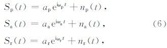
(1)对3个数据块采用OSE和PSA相结合的方法计算，即可获得三个新的观测序列S_pi(t)、S_ai(t)、S_ri(t)(i=1，2，3)；分别计算每个数据块对 应于三个单线态的积谱密度P_pi(ω)、P_ai(ω)、P_ri(ω)(i=1，2，3)，并剔除其中一些显著的已知信号，则₁S₁三重分裂谱线的积谱密度可以表示为 P_j(ω)=P_ji(ω)(j=p，a，r)，且分别对应于三个分裂谱线m=-1，m=0和m=+1.

(2)只采用PSA方法直接计算各数据块的积谱密度P_i(ω)=[ P_ij]^1/9(i=1，2，3)，P_ij表示第i 个数据块中第j个残差序列的功率谱密度(j=1，2，…，9)，同样剔除其中一些显著的已知信号，则残差序列最终的积谱密度为P(ω)=[P_i(ω)]^1/3.

图 4为采用方案1处理后的积谱密度.类似于 Smylie(1992)、Courtier等(2000)和Ding和Shen(2013)，我们采用五次多项式拟合3个分裂谱线的积谱密度来评估背景噪声水平.从图中可以看出，一些已知信号(包括大气潮汐信号S₄以及一些残余潮汐信号MN₄、M₄、SN₄、N₄、MS₄、K₃)对目标频段的噪声水平有影响.通过剔除这些已知信号，背景噪声水平明显降低，一些微弱的共振信号有所增强.

图 4

Fig. 4

图 4 采用方案1处理后的原始积谱密度(蓝色曲线)与剔除某些已知信号后的积谱密度(红色曲线) 积谱密度曲线中央的蓝色虚线为原始积谱密度的背景噪声水平估计，两侧的蓝色虚线为相应的95%置信水平(CI)曲线；积谱密度曲线中央的红色虚线为剔除某些已知信号后的积谱密度的背景噪声水平估计，两侧的红色虚线为相应的95% CI.垂直虚线表示大气潮信号S4—S7， 箭头表示某些已知的残余潮汐信号.Fig. 4 Original product spectra (blue curve) and demodulated product spectra (red curve) after using the scheme 1 Blue dashed curves in the middle of the product spectra denote estimates of background noise levels of original product spectra, Blue dashed curves on either side show corresponding 95% confidence interval (CI). Red dashed curves in the middle of the product spectra denote estimates of background noise levels of demodulated product spectra. Blue dashed curves on either side show the corresponding 95% CI. Atmospheric tidal signals of S4—S7 are indicated by vertical dotted gay lines. Arrows indicate some well-known nonlinear tides.

在检测₁S₁三重分裂信号时，可能会出现若干组谱峰(分别对应m=-1、m=0、m=+1的谱线分裂)，它们均有可能是Slichter 模₁S₁的三重分裂谱线.为判断某一谱峰是否为可能的₁S₁单线态，我们参照Ding和Shen(2013)基于OSE的特征设置了两个准则：(1)该谱峰振幅P_s(ω_i)(ω_i为该谱峰对应的频率)要高于95%的置信水平(CI)曲线；(2)其他两个积谱密度中相应频率的谱峰振幅 P_q(ω_i)(q=p，a，r; q≠s)要小于80%的CI曲线.严格满足以上两个准则，则认为该谱峰可能是某一₁S₁单线态.

图 5给出了在0.16~0.28cph频段内采用方案1计算剔除某些已知信号后的积谱密度.从图中可以清楚地看到，有8个谱峰同时满足两个准则，图中用不同颜色的竖线和箭头表示出了各谱峰在该频段内的位置和相应频率，其中对应于m=-1单线态信号的可能谱峰有1个，对应于m=0单线态信号的可能谱峰有5个，对应于m=+1单线态信号的可能谱峰有2个；有5个谱峰虽然满足第一准则，但不满足第二准则；因此，尽管它们的信噪比较高，我们认为这几个谱峰可能是台站的背景噪声信号，也可能是某些与其他地球物理和地球动力学因素有关的信号(孙和平等，2004; 徐建桥等，2005).此外，在三个积谱中未发现任何谱峰的周期对应于Smylie等(1992)声称检测到的₁S₁三重分裂谱线的周期.

图 5

Fig. 5

图 5 采用方案1计算且剔除某些已知信号后的功率谱密度 黑色虚曲线为背景噪声水平估计，蓝色和红色虚曲线分别对应95%和80% CI曲线.黑色竖直虚线表示只满足第一个准则的相应谱峰；不 同颜色的竖直虚线表示同时满足两个准则的谱峰，相应颜色的箭头表示这些可能信号在频谱密度中出现的位置.其中， 红色竖直虚线对应1S1 单线态信号m=-1，蓝色竖直虚线对应1S1单线态信号m=0，绿色竖直虚线对应1S1单线态信号m=+1.Fig. 5 Demodulated product spectra after using the scheme 1 Black dashed curves denote estimates of background noise levels. Blue and red dashed curves correspond to 95% and 80% CI curves. Vertical black dashed lines denote the corresponding peaks that only satisfy first criterion. Vertical solid dashed lines with different colors denote corresponding peaks that satisfy both criteria. Corresponding color arrows denote spectra with possible signals appearing. Red dashed line corresponds to singlet m=-1 of 1S1. Blue dashed line corresponds to singlet m=0 of 1S1. Green dashed line corresponds to singlet m=+1 of 1S1.

我们重点关注可能频段(0.17~0.26cph)内的 积谱密度，并采用Savitaky-Golay平滑滤波(Savitzky and Golay，1964)方法来处理相应频段的积谱密度，以凸显信噪比高的信号，而压制信噪比低的信 号.图 6给出了经过平滑处理后的积谱密度及其相应的CI曲线.对比图 5和图 6，平滑处理前后积谱密度曲线整体上变化不大；图 5中与噪声信号非常接近的一个可能谱峰信号经过平滑后，基本与噪声信号的频率一致，说明该谱峰实际上是由于该噪声信号谱峰宽度较大，剥离在不同单线态频谱中尖峰值可能发生偏移.图 6表明，共有7个谱峰同时满足上述两个准则，也即这7个谱峰可能为₁S₁三重分裂信号.用P、A、R分别表示₁S₁三重分裂谱线，采 用AR方法估计7个谱峰的中心频率ω₀，表 2给出了经过平滑处理后检测到的7个可能谱峰相应的中心频率ω₀和其对应的周期T₀.虽然检测到了可能为₁S₁单线态的谱峰，但没有找到一组谱峰符 合₁S₁三重分裂的分裂宽度，说明这7个谱峰中可能只有2个或更少的谱峰为可能的₁S₁单线态，其他几个信噪比较高的背景噪声信号对₁S₁单线态干扰较大.

图 6

Fig. 6

图 6 经过平滑后的积谱密度(只关注0.17~0.26cph的可能频段) 检测到的谱峰与图5相应频率的谱峰基本一致.黑色竖直虚线表示只满足第一个准侧的相应谱峰；不同颜色的竖直虚线表示同时满足两个准侧的谱峰，相应颜色的箭头表示这些可能信号在积谱密度中出现的位置.Fig. 6 Product spectra after smoothed (only concerning possible frequency band 0.17~0.26 cph) Detected peaks are the same as the peaks of the corresponding frequency in Fig.5. Vertical black dashed lines denote the corresponding peaks that only satisfy the first criterion. Vertical dashed lines with different colors denote the corresponding peaks that satisfy both criteria. Corresponding color arrows denote spectra with possible signals appearing.

表 2(Table 2)

表 2 采用方案1检测到的7个谱峰的中心频率及其对应周期的估计结果 Table 2 Central frequency and period estimates of observed 7 peaks using the scheme 1 谱峰 ω 0(cph) T 0(h) P 0.171505±2.09×10 -5 5.83073±7.10×10 -4 A A1 0.175431±7.85×10 -5 5.70026±2.55×10 -3 A2 0.177047±6.99×10 -5 5.64822±2.23×10 -3 A3 0.191714±2.97×10 -5 5.21611±8.08×10 -4 A4 0.218056±2.57×10 -5 4.58597±5.39×10 -4 R R1 0.247609±2.55×10 -5 4.03863±4.15×10 -4 R2 0.258569±2.92×10 -5 3.86743±4.37×10 -4

表 2 采用方案1检测到的7个谱峰的中心频率及其对应周期的估计结果 Table 2 Central frequency and period estimates of observed 7 peaks using the scheme 1

为完善₁S₁三重分裂谱线的观测结果，我们基于Smylie等(1993)给出的PSA方法(即方案2)来检测可能的弱共振信号，并以五次多项式拟合平滑后的积谱密度作为相应频段上背景噪声，以谱峰峰值大于95%的CI作为可检测信号的最低能量限制.按照此准则，我们在0.17~0.26cph频段内一共检测到了13个谱峰(Spectral Peak，SP)，并用SPi(i=1，2，…，13)按照频率由高到低表示相应的谱峰.图 7给出了平滑前后剔除某些已知信号后的积谱密度，表 3给出了采用方案2检测到的13个谱峰的中心频率ω₀及其对应的周期T₀ .从图 7可以看出，经过平滑处理后，一些振幅较高而信噪比不大的谱峰得到明显压制；而一些信噪比不高的信号，经

图 7

Fig. 7

图 7 采用方案2计算的积谱密度 黑色曲线为剔除了某些已知信号后的积谱密度，红色曲线为剔除了某些已知信号和平滑后的积谱密度；积谱密度曲线中央的黑色虚线为背景噪声水平估计，上下两侧的蓝色虚线为相应的95% CI曲线.Fig. 7 Product spectra using the scheme 2 Black curves denote the demoded product spectra. Red curves denote corresponding smoothed spectra. Black dashed curve in the middle of product spectra curve is estimate of background noise level. Blue dashed curves on either side are corresponding 95% CI curves.

表 3(Table 3)

表 3 采用方案2检测到的13个谱峰的中心频率及其对应周期的估计结果 Table 3 Central frequency and period estimates of observed 13 peaks using the scheme 2 谱峰 ω 0(cph) T 0(h) SP1 0.170826±1.93×10 -5 5.85391±6.60×10 -4 SP2 0.174681±2.02×10 -5 5.72473±6.63×10 -4 SP3 0.175258±2.28×10 -5 5.70588±7.43×10 -4 SP4 0.178269±1.94×10 -5 5.60950±6.10×10 -4 SP5 0.180781±2.40×10 -5 5.53157±7.34×10 -4 SP6 0.184193±3.82×10 -5 5.42909±1.12×10 -3 SP7 0.195345±1.95×10 -5 5.11914±5.12×10 -4 SP8 0.197837±2.19×10 -5 5.05466±5.61×10 -4 SP9 0.198754±1.93×10 -5 5.03135±4.89×10 -4 SP10 0.210366±2.28×10 -5 4.75363±5.15×10 -4 SP11 0.241721±2.03×10 -5 4.13700±3.47×10 -4 SP12 0.249664±2.13×10 -5 4.00538±3.41×10 -4 SP13 0.256722±1.96×10 -5 3.89527±2.97×10 -4

表 3 采用方案2检测到的13个谱峰的中心频率及其对应周期的估计结果 Table 3 Central frequency and period estimates of observed 13 peaks using the scheme 2

过平滑处理后依然可能达到我们设定的大于95%的CI可检测准则.比较两种方案的检测情况，可以看出基于OSE方法检测到的谱峰与基于PSA方法检测到的谱峰中心频率相差较大.

综合考虑前人的理论计算结果，Slichter模的 周期约为3~6 hours，分裂宽度约为15~40 minutes(Dahlen and Sailor，1979; Crossley，1992; Hinderer and Crossley，1993; Rochester and Peng，1993; Peng，1995，1997; Denis et al.，1997; Rogister，2003; Smylie et al.，2009; Rosat，2011)； 而对于PREM模型，Slichter模的中心周期约为5.2~5.3 h(Peng，1995，1997; Denis et al.，1997; Rogister，2003; Smylie et al.，2009; Rosat，2011). 鉴于OSE方法检测₁S₁三重分裂信号更为严格，我们以OSE方法检测的结果为基础，结合两种方案检测结果，并参照理论模型结果，找到了唯一一组可能的三重分裂信号(见表 4)，它们是基于OSE方法检测到的2个谱峰P(m=-1：5.8307±7.1×10^-4h)、A3(m=0：5.2161±8.1×10^-4h)和基于PSA方法检测到的1个谱峰SP10(m=+1：4.7536±5.2×10^-4h)，这三个谱峰所对应的周期与Crossley(1992)、Rochester和Peng(1993)、Peng(1997)和Rogister(2003)基于PREM模型给出的理论周期之间的相对误差约1.48%，与Ding和Shen(2013)建议的“可能的观测结果”之间的相对误差约为0.59%；其中，m=+1信号的强度明显高于m=0和m=-1信号.

表 4(Table 4)

表 4 Slichter模的理论预测周期及本文观测周期(单位：h) Table 4 Predicted and observed periods of Slichter modes (unit: h) Model m=-1 m=0 m=+1 Dahlen and Sailor (1979) 1066A 6.5980 5.8044 5.1663 Smylie(1992) 1066A 2.8247 2.7023 2.6035 CORE11 3.7195 3.5056 3.3432 Crossley(1992) PREM 5.9792 5.3104 4.7667 1066A 5.0161 4.5329 4.1270 Crossley et al. (1992) 1066A 5.0140 4.5338 4.1284 Rochester and Peng(1993) PREM 5.9697 5.3017 4.7595 Peng(1997) PREM 5.9782 5.3087 4.7642 Rieutord(2002) 1066A 4.687 4.255 3.894 Rogister(2003) 1066A 5.024 4.529 4.129 PREM 5.991 5.309 4.770 Ding and Shen(2013) observed 5.894±1.7×10 -3 5.208±2.3e-3 4.728±2.1×10 -3 This paper observed 5.8307±7.1×10 -4(OSE) 5.2161±8.1×10 -4(OSE) 4.7536±5.2×10 -4(PSA)

表 4 Slichter模的理论预测周期及本文观测周期(单位：h) Table 4 Predicted and observed periods of Slichter modes (unit: h)

(1)基于2004年苏门答腊地震后GGP观测网中9台超导重力仪13200h的连续重力观测数据，将 EEMD作为滤波器处理常规预处理后的重力残差，提取其中包含目标频段的IMFs，作为最终各台站的重力残差，有利于提高信噪比.结合时间域内的OSE方法和频率域内PSA方法，迭积了9个超导重力台站重力残差的功率谱密度，并对积谱采用剔除某些已知信号和平滑处理；参照Ding和Shen(2013)设置的两个检测准则，并依据Slichter模的分裂特征选取了两个候选谱峰，对应于Slichter模的两个单线态信号m=-1和m=0.只采用频率域内PSA方法处理相同的重力残差序列，我们找到13个微弱谱峰，对照基于OSE方法得到的两个单线态并兼顾理论分裂宽度，从中选取了一个候选谱峰，对应于Slichter模的单线态信号m=+1.结合两种处理过程的检测结果，我们探测到了一组结果(5.8307±7.1×10^-4 h，5.2161±8.1×10^-4 h，4.7536±5.2×10^-4 h)，不仅与Crossley(1992)、Rochester和Peng(1993)、Peng(1997)和Rogister(2003)基于PREM模型给出的理论周期很接近，而且也与 Ding和Shen(2013)的探测结果非常接近.需要指出，本研究与Ding和Shen(2013)的研究完全独立，尽管检测Slichter模的方法相同，但采用的数据源不同，且数据预处理的方法也不同.这一独立探测结果，从某种意义上说，证实了Ding和Shen(2013)探测到的“可能的Slichter 模三重分裂值”.

(2)最后需要指出，Rosat和Rogister(2012)认为，只有震级超过M_W9.7的大地震才能激发出足以观测得到的Slichter模三重分裂信号，但他们的结论有待商榷，因为一个显然的事实是，通过多台站叠积技术可有效放大全球性信号，但他们忽视了这一点.不过，毫无疑问，由于我们并不能象探测如₂S₁模态那样看到清晰、明显的三个谱峰，因此，我们尚无法判定本文所检测到的三个谱峰是否一定是地球内核的平动振荡信号.此外，还有一些谱峰信号其原因不明，这些信号是否由地球内核平动振荡所致，还是与其他一些地球物理过程(或事件)如海浪、潮汐效应等有关，还有待进一步研究.