 2016, Vol. 59


We first use the 1-D spring-slide block model governed by the R-S law to simulate earthquake cycle and triggered seismic activities caused by different static shear stress changes. Then we compare the simulation results separately with the solutions given by the Dieterich model and the Coulomb failure model, and the differences between our numerical simulation and the Dieterich and Coulomb models are discussed.
Our results indicate that, at postseismic/afterslip stage and interseismic stage, the advanced or delayed time is constant and increases with the absolute values of static stress load growing. Moreover, the ratio of the advanced and delayed time is about 1.0. These phenomena could be predicted by both Dieterich's model and Coulomb failure model, and the difference between current simulation and two models is no more than 10% of the calculated results of two models. At preseismic stage, the simulated result has distinctive features comparing severally with two models. First, when shear stress loaded at preseismic stage, all the results from the simulation differ with the results from the Coulomb failure model, and the ratio of the advanced and delayed is lower than 1.0 which is in contrast with the conclusion from the Coulomb failure model. While loaded positive static shear stress changes, the Dieterich's model and the numerical simulation give the much similar results, and the difference between the Dieterich's model and numerical simulation is less than 7% of calculation of Dieterich's model, and even approach to zero. The results are the same as above when the absolute value of negative static shear stress changes are small, with difference less than 14% of outcome of Dieterich's model. But while the absolute value of negative static shear stress changes become larger, the simulated result is more than that derived from the Dieterich model, and can reach to 35 times or more. This significant difference caused by the large negative static stress loading is due to that the condition Ω=δθ/dc>>1 used in the Dieterich's approach doesn't satisfy anymore. Therefore, the Dieterich model fails in such an extreme case.
The numerical solutions show that without parameters changing, the advanced or delayed time strongly depends on both the onset time when static shear stress is applied and the amplitude of the applied shear stress. Moreover, the variation of the advanced or delayed time for positive or negative static shear stress which absolute values are equal isn't same. Compared with our numerical simulation, the Dieterich model gives a more proper description of the time advance or time delay than that resulted from the Coulomb failure model which is a very popular model used in the earthquake forecasting model development. And the Dieterich model can show the different variation of the advanced or delayed time for positive or negative static shear stress.
预测中至强震的发生时间、地点和震级是震源力学研究的终极目标.在地震灾害的防御和减灾工作的实施过程中,对地震重复发生时间间隔的估算也是目前我们所面临的一个重大挑战.对于地震重复发生时间的认识,现今广泛认可的控制模式可归结为:未来发震断层的构造剪应力加载速率,断层本身的摩擦性质,周边地震对未来发震断层的影响(Stein,1999).中强地震可以构成对区域应力场的扰动,这样的扰动包含了静态和动态应力变化,以及地壳内部流体压力的变化,岩石的塑性变形.因此,断层上的静态应力加载或卸载可以导致断层演化周期的改变,出现断层失稳时间的提前或延后.最为普遍的一个现象就是围绕发震断层在内的区域地震活动性的增加(触发地震的产生)或地震活动性的下降(地震影区)(King and Cocco,2001).在Coulomb应力失稳模型(下文简称Coulomb模型)中(Stein et al.,1997),断层失稳时间提前或延后量Δt正比于ΔCFF/  ,ΔCFF=Δτ+μ′Δσ,其中μ′为有效摩擦系数(King et al.,1994),Δτ和Δσ分别为剪应力和正应力变化量,若Δσ=0,Δt为ΔCFF/ =Δτ/ ,为远场构造剪应力加载速率(Gomberg et al.,1998; Harris and Simpson,1998; Perfettini et al.,2003).图 1给出了受静态应力扰动后Coulomb模型断层失稳示意图.从图中可以看到,当断层上的累积剪应力大于或等于断层摩擦强度时,断层发生突发失稳.因此,当 给定时,应力扰动后的断层失稳时间的提前或延后量Δt只同ΔCFF的绝对大小有关,而同扰动的加载时刻无关.另外,从图 1中可以得到,静态应力扰动量与时间提前或推后量Δt满足线性关系.也就是说,只要应力加载的ΔCFF不会直接使得断层上的剪应力和正应力满足Coulomb破裂准则,那么无论是在断层演化的那一阶段,对断层施加的静态库伦应力变化ΔCFF,只要其绝对值相同,那么时间的提前或延后量Δt都是相同的.考虑到断层演化的复杂性,这一时间变化的描述显得过于简单.例如,利用实际地震数据,Harris和Simpson(1998)指出Coulomb模型并不能很好地确定地震的延后时间.虽然Coulomb模型已成功地应用于包括L and ers地震(Harris and Simpson,1992)和North Anatolian断层活动(Stein et al.,1997; Parsons et al.,2000)在内的许多地震序列的模拟和未来地震发生概率的计算,但其局限性是非常明显的(Hardebeck,2004; Parsons,2005a; Gomberg et al.,2005b).例如,(1)Coulomb模型无法对触发余震随时间的衰减特征给出定量化描述;(2)虽然Δt=Δτ/用于未来地震发生条件概率的计算,但忽略了断层演化过程中不同应力加载时间下Δt取值的变化.事实上,通过研究触发地震的力学机制,我们可以推测各个断层发震的可能性,实现基于物理的地震危险性评估(Freed,2005).另外,对地震触发机制的深入研究,我们可以鉴别不同震源模型以及其控制参数,了解和推测震源的实际演化过程(Gomberg et al.,2000).
 | 图 1 Coulomb模型中破裂时间的提前或推后. 当 给定时,Δt只同ΔCFF的大小相关,与加载时刻无关.当|ΔCFF|给定时,时间的提前或延后量是相等的 Fig. 1 Schematic illustration of the time advance or delay for the Coulomb failure model. When , the remote loading of shear stress rate, is given, Δt, the time advance or delay depends only on the amount of ΔCFF. The onset time while the static shear stress is applied doesn′t affect Δt. In this model, the advanced or delayed times are the same if |ΔCFF| is given |
自弹性回跳学说诞生以来,有关地震成因力学机制的研究得到了广泛和深入的开展.对发震断层的演化过程,目前地震学家比较一致的认识是(Stein and Wysession,2003):在断层完整演化过程中,断层的滑动经历了四个明显不同阶段:(1)闭锁阶段(Interseismic Stage);(2)自加速阶段(Preseismic Stage,Nucleation);(3)同震相(Coseismic Phase);(4)震后松弛/滑移阶段(Postseismic/Afterslip Stage).受地震观测数据的限制,我们对于每个阶段中的断层摩擦动力学过程及其复杂性知之甚少.事实上,岩石力学实验表明,断层摩擦过程直接同断层内部的滑移速率和状态有关.滑移速率与状态相依赖的摩擦本构关系(Rate- and State- Dependent Friction:简称R-S摩擦定律)已普遍用于对发震断层孕育、成核及发震深度约束的研究(Scholz,1998).在此本构关系的框架下,近期有关断层演化,地震复发周期,以及触发地震成因机制的数值分析和理论研究在全球范围内得到了广泛关注(Perfettini and Avouac,2004a,2004b; Kaneko et al.,2010; Barbot et al.,2012; Kame et al.,2013a).而关于静态应力扰动后断层失稳的时间提前或推后的论述则最早来自Dieterich(1992,1994)余震触发机制的解析模型(下文简称Diererich模型).在此模型中,余震发生于各自断层演化期中的自加速阶段,因此若不考虑正应力的变化,那么时间提前或延迟量Δt只有在应力加载时刻t0远离断层失稳时刻时才有Δτ/ (Gomberg et al.,1998; Hardebeck,2004).Perfettini等(2003)在2-D断层摩擦失稳的数值模拟中,进一步讨论了在断层上正应力发生变化的条件下对断层失稳时间的估算,结果表明当加载时刻处于断层演化周期前90%的情况下,时间提前或延迟量接近ΔCFF/,即等于Coulomb模型所估算出的值,而在地震演化周期的后10%,则可出现显著的不同.Gomberg等(1997,1998,2000)的研究中也有相似的结果.
在本文中,利用R-S摩擦定律,从1-D弹簧-滑块模型出发,数值模拟在不同加载时刻,不同大小静态应力扰动(本文中暂不考虑正应力变化)下,对应的发震时刻(断层失稳的时间)提前或推后的变化情况.通过模拟计算可以发现在R-S摩擦定律控制下,失稳时间提前或推后量的大小依赖于静态应力扰动的大小和加载时刻,而且正、负向静态应力扰动后对应了不同失稳时间提前或推后的变化情况;另一方面,通过将上述结果分别与Coulomb模型和Dieterich模型的计算值分别进行比较和讨论后,可以证明Coulomb模型中提出的断层失稳时间的提前或推后的解析表达式仅可以描述震后松弛/滑移阶段(Postseismic/Afterslip Stage)和闭锁阶段(Interseismic Stage)的情况,而Dieterich模型则能完整地给出断层演化不同阶段受不同静态应力扰动后断层失稳时间的提前或推后量的变化情况,并能解释正、负向静态应力扰动的差异性.
2 理论模型2.1 速率-状态摩擦定律(R-S摩擦定律)R-S摩擦定律为我们提供了一个基本的物理途径用以定量化描述断层内部复杂的摩擦情况.该摩擦关系是由岩石力学实验结果所总结出的定律,它已成为研究地震成因和断层演化力学机制的重要理论基础,用以描述几乎所有观察到的同震滑移和震间断层响应,并被广泛地用于描述地震行为规律性的变化(Marone,1998).目前使用最广泛的R-S摩擦定律为Dieterich定律(Segall,2010),即
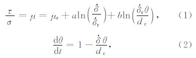
 分别为断层面上的滑动位移和滑移速率.r是参考速率;μr是以r稳定滑动时的摩擦系数;θ为状态变量,表示了凹凸体的平均接触时间,也就是从凹凸体接触形成至今的平均时间(Dieterich,1979).a和b是反映介质性质的常数,由实验数据得出,其取值范围在0.01左右.其中,a为“直接影响”系数,它决定速率变化引起的摩擦强度变化,b为“演化影响”系数,它控制状态演化所引起的摩擦系数的变化(Bhattacharya and Rubin,2014).当(a-b)≥0时,断层的摩擦过程表现为速度强化,此时断层的滑动总是稳定的,而当(a-b)<0时,断层的摩擦过程表现为速度弱化,此时断层的滑动可以是条件稳定,也可以不稳定,对应了地震发生时的断层失稳态(Scholz,1998).dc为临界滑动距离,表示了彻底改变摩擦面接触状态所需的滑动距离(Marone,1998).2.2 1-D弹簧-滑块模型
除了R-S摩擦定律,为了模拟断层摩擦应力随时间变化的特征,我们还需要一个描述摩擦面和其周围介质之间弹性作用的断层力学模型.为了定性地说明问题,通常采用1-D弹簧-滑块模型,其断层上的加载应力τ可以表示为
 b为远场滑移加载速率,通常为一常数.由此远场剪应力加载速率可表示为b=kb.公式(3)也可改写为
 (0),τ(0)和θ(0)的情况下,联立求解方程(1)、(2)和(3)或(1)、(2)和(4),就可以模拟断层演化过程,其中,当→∞时发生破裂失稳.为了避免→∞这一非物理现象的发生,通常在数值求解过程中加入辐射衰减项(Bizzarri,2012),如对(3)式在时域求导,可得以下方程:
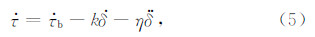
假定作用于断层上的正应力σ保持不变,根据Dieterich(1994)可得加载静态应力扰动Δτ前后断层滑动速率1和2满足

如图 2,定义加载时刻为t0,未扰动时从t0时刻到断层模型失稳所需的时间为T,扰动后从t0时刻到断层模型失稳所需的时间为f.定义Ω=θ/dc,则在Ω远远大于1的条件下,Dieterich(1992,1994)利用公式(1)、(2)和(4)推导出当初始时刻滑移速率为0时,断层的失稳时间T(未经应力扰动)为

 0的增加,T和f则相应地减小,说明对于Dieterich模型,滑移速率是随时间不断增大的.另外,当Δτ>0时,f小于或接近于T,表明正向的静态应力扰动使得失稳时间发生提前,即Δt=T-f;而当 Δτ<0 时,f大于T,即负向的静态应力扰动使得失稳时间发生推后,即Δt=f-T.显然,f也可写为T的函数(下文中讨论).
 | 图 2 正向静态应力扰动示意图. 其中实线表示未扰动时的演化,而虚线表示存在扰动时的演化.其中t0表示施加静态应力扰动的时刻,T表示未扰动时从t0时刻到断层模型失稳所需的时间,f表示扰动后从t0时刻到断层模型失稳所需的时间 Fig. 2 Schematic illustration of the slip velocity evolution with and without positive static stress perturbation. The solid and dashed lines show the unperturbed and perturbed response, respectively, and t0 is the onset time of the shear stress perturbation. T and f denote the time from t0 to the unperturbed failure time and the time from t0 to perturbed failure time, respectively |
结合公式(1),(2)和(4)或(1),(2)和(5),采用四阶龙格库塔算法(4th-Order Runga-Kutta Algorithm),我们可以求出不同参数条件下1-D断层演化特征.图 3给出了加入辐射衰减项后模拟得到的包括滑动位移、滑移速率和应力变化在内的断层演化过程.不难看出在模拟计算开始的0~160年里,计算结果与之后时间段的结果并不相同,这是由初始参数(0),τ(0)和θ(0)的影响造成的,而之后时间段的演化则反映了介质参数控制的1-D断层模型本身的演化特征,因此之后的分析中都不考虑0到160年的演化情况.图 3a给出了滑移速率的变化特征.滑移速率随时间的变化呈现出了明显的周期性特征,其复发周期的尺度由图中Tr表示,断层的失稳时刻则对应于滑移速率达到0.14 m·s-1的时刻,即达到地震同震滑移时速率的时刻.一般来说,Tr的长短主要取决于弹簧刚度系数k和远场加载速率,但本文的重点在于静态应力扰动对失稳时刻的影响,所以对于Tr的影响因素在此不做更深入的讨论.另外,在每一个周期内,大约95%Tr内滑移速率很小(<10-8m·s-1),可以认为断层是静止的,而在很短的时间内滑移速率迅速增大,直至失稳.同样地,在图 3c中,失稳前断层的位移大小均近似为零,仅仅在极短时间的失稳过程中产生了滑动位移.这些特征均与断层运动的黏滑机制一致.图 3b 则显示出断层摩擦应力的最高值和最低值保持不变,表明了在每次滑块失稳后,静态应力降是相同的.进而也反映了每次失稳事件的发生,相应的模拟地震震级是完全相同的.因此,利用R-S摩擦定律和1-D弹簧-滑块模型可以模拟理想地震的重要演化特征.对于断层摩擦过程随时间的变化,图 3e中则显示出了四个主要明确的阶段.模拟结果显示出:断层闭锁阶段(Interseismic Stage)至少占据了总的演化周期Tr的80%,而自加速阶段(Preseismic Stage,Nucleation)、同震相(Coseismic Phase)和震后松弛/滑移阶段(Postseismic/Afterslip Stage)三个阶段仅仅只有20%Tr(如图 3e).从图 3d中不难看出对于模拟计算,仅在自加速阶段和同震相阶段才能满足Ω远远大于1,则与前述一致,Dieterich模型仅能用于描述断层处于自加速阶段和同震相阶段(时间很短可忽略)时受到静态应力扰动后的演化特征,因此有必要模拟计算出其他阶段受到静态应力扰动后断层演化过程发生的变化,并与Dieterich模型进行对比,以明确Dieterich模型的局限性.
 | 图 3 未受扰动时1-D断层模型的演化 (a) 断层速率的演化图,其中Tr为断层模型的完整演化周期; (b) 断层所受摩擦应力的演化图; (c) 断层滑移距离的演化图; (d) 断层模型中Ω= θ/dc在一个周期内的变化情况,其中曲线的色度表示了曲线上某一点所处的时刻占整个演化周期的比例; (e) 断层演化在速率-应力相平面上的相图,其中曲线的色度表示了曲线上某一点所处的时刻占整个演化周期的比例. Fig. 3 Frictional responses of the 1-D fault model(a) Slip velocity evolution during a multi-seismic cycle. Tr represents a typical earthquake recurrence period. (b) Frictional shear stress variations on the fault during a multi-seismic cycle. (c) The stick-slip motion related time history of slip displacement. (d) The variation of Ω= θ/dc in a seismic cycle, and the color represent the percentage of the cycle period. (e) Plot of the closed trajectory (cycle) in the phase plane, and the color represent the percentage of the cycle period.
|
前人对于静态应力扰动的研究主要集中在正向静态应力扰动(Δτ>0)对断层演化的影响(Gomberg et al.,1998; Gomberg et al.,2000; Gomberg et al.,2005a; Kaneko and Lapusta,2008),而对负向静态应力扰动(Δτ<0)情形下时间推后量Δtd同时间提前量Δta之间差异性的讨论相对较少.2003年,Perfettini等讨论了2D断层模型受静态应力扰动后时间提前和推后量之间的关系,他们的结果表明两者之间的比值为一震荡的曲线.因此,我们有必要从数值模拟入手,探讨其差异性出现的缘由以及同Coulomb模型和Dieterich模型作对比.表 1给出了本文在计算模拟中所使用的模型参数值(主要取自Kame et al.,2013b).
| | 表 1 模拟计算时使用的模型参数值 Table 1 Parameters used for the numerical calculation and simulation |
在模拟计算中,正向静态应力扰动的取值分为Δτ= 1,2,5,10和15 MPa,分别在整个演化周期内的不同时刻t0加载,这样就可以计算出不同时刻t0对应的未扰动时失稳时间T和扰动后失稳时间f,然后就能得到失稳时间的提前量Δt=T-f,接着可以分别绘出模拟计算结果与Coulomb模型和Dieterich模型的对比图和差异性分析图(图 4).首先是模拟结果和Coulomb模型的对比,如图 4a和图 4c,不难看出,对于正向加载(Δτ>0),在断层模型演化早期(震后松弛/滑移阶段和闭锁阶段)加载,Coulomb模型给出的时间提前量(虚线)比模拟计算的(实线)结果小,而且两者的差值随Δτ的增大而增大,不过其差值不超过Coulomb模型的10%(图 4c),说明两者在断层模型演化早期阶段基本保持一致.而在演化后期的应力加载,模拟结果得到的时间提前量随加载时刻的推后而不断减少趋于零,即当t0→ Tr,f → 0,明显不同于Coulomb模型给出的时间提前量值.而且两者相近的时间段也随着应力扰动量的增大,由80%的演化周期Tr减小至50%的演化周期Tr.
 | 图 4 不同正向静态应力扰动(Δτ>0)对应的加载时刻和失稳时间提前量Δt关系及差异分析 其中t0表示加载时刻,Tr表示模型的演化周期. (a) 模拟计算结果(实线)与Coulomb模型(虚线)的比较; (b) 模拟计算结果(实线)同Dieterich模型(虚线)的比较; (c) Coulomb模型与模拟计算的差值,Difference=(ΔtCoulomb-ΔtSimulation)/ΔtCoulomb; (d) Dieterich模型与模拟计算的差值,Difference=(ΔtDieterich-ΔtSimulation)/ΔtDieterich. Fig. 4 The advanced times after applying different positive static stress perturbations (Δτ>0) as a function of the onset time of the stress perturbations t0 is the onset time of the application of the stress perturbation. Tr is the cycle period. (a) A comparison between the simulations (solid lines) and the results derived from Coulomb failure model (dashed lines); (b) A comparison between the simulations (solid lines) and results derived from Dieterich model (dashed lines); (c) The differences between the Coulomb failure model and simulation with given different stress perturbations, and the Difference=(ΔtCoulomb-ΔtSimulation)/ΔtCoulomb; (d) The differences between the Dieterich model and simulation, and the Difference=(ΔtDieterich-ΔtSimulation)/ΔtDieterich. |
事实上,根据Rubin和Ampuero(2005)的结果,可知在模型的演化早期,满足Ω远远小于1,从而有下式:
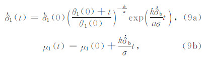
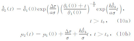 2(0)=1(0)exp(Δτ/aσ),μ2(0)=μ1(0)+Δτ/aσ和θ2(0)=θ1(0)的演化情况一致,如图 5.这就说明在演化早期加载后,模型演化的失稳时刻是不变的,即失稳时间提前量Δt是不变的.另外正向静态应力扰动会令加载前后Ω之比为Ω2(t0)/Ω1(t0)=exp(Δτ/aσ),也就是说正向静态应力扰动越大,加载后Ω就越接近1甚至超过1,而不再满足上述条件,因此,静态应力扰动越大失稳时间提前量Δt为定值的时间就越短.
 | 图 5 在震后松弛/滑移阶段和闭锁阶段加载静态应力扰动时模型的演化情况(点线)与初始条件改变时演化情况(实线)的对比. 其中虚线表示未加载扰动时模型的演化情况.加载时刻为t0=0.5Tr,静态应力扰动为Δτ=5 MPa Fig. 5 A comparison of the temporal slip velocity evolution (dotted line) while the static stress perturbation is applied at postseismic/afterslip stage or interseismic stage and the temporal slip velocity evolution (solid line) with a changing of the initial conditions. The dashed line represent the temporal slip velocity evolution without static stress perturbation. The triggering time t0 satisfies t0=0.5Tr, and the static stress perturbation is Δτ=5 MPa |
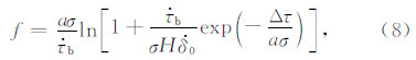
由公式(7)和(8),可知在Dieterich模型中,应力扰动后失稳时间f和未扰动时失稳时间T满足以下关系(Kaneko and Lapusta 2008):
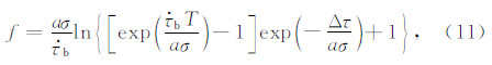
 b,那么当T/ta远远大于1时,Δt近似等于Δτ/b,如图 4b 所示,这与Coulomb模型的结果一致,即在演化早期模拟计算结果(实线)和Dieterich模型(虚线)的差值较大,为一定值,且随Δτ的增大而增大.当未扰动时失稳时间T满足T远远小于ta时,即加载时刻位于断层模型演化末期时,(15)式近似可得f≈Texp(-Δτ/aσ),进而有Δt≈T[1-exp(-Δτ/aσ)],那么随着T减小,即t0逐渐接近失稳时刻时,Δt就越小,而趋于零,如图 4b中虚线的变化情况.Dieterich模型的两条渐进线Δt=Δτ/b和Δt=T[1-exp(-Δτ/aσ)]交点的横坐标为t0/Tr=1-Δτ/{bTr[1-exp(-Δτ/aσ)]},若把t0/Tr作为Δτ的函数,通过求导可以得出随Δτ的增大t0/Tr是减小的,也就是说两条渐进线的交点会逐渐偏向演化早期,这就表明随Δτ的增大,Dieterich模型得到的Δt的变化曲线偏离常数Δt=Δτ/b的时间点在逐步提前(图 4b),这与模拟结果的情况一致.对于断层模型,显然在演化后期,其状态变量和速率就开始满足Dieterich模型的条件Ω远远大于1,而且正向静态应力扰动Δτ越大,就越使得扰动后的Ω满足这一条件,于是一方面在演化后期有模拟计算和Dieterich模型结果的差值相对很小;另一方面,随Δτ增大,上述差值从常数衰减的时间就越早,衰减幅度也越大.总体上看,虽然Dieterich模型要求Ω远远大于1,即Dieterich模型仅能描述自加速阶段断层受扰(或未受扰)的演化情况,但对于正向静态应力扰动,模拟计算结果与Dieterich模型结果的差值最大不超过Dieterich模型给出值的9.5%,也就是说,即使是早期演化阶段,Dieterich模型对失稳时间提前量的估计和模拟计算结果也是一致的.3.2 负向静态应力扰动
和正向静态应力扰动相对应,我们选择的扰动值为Δτ=-1,-2,-5,-10和-15 MPa,相应的加载时刻t0和失稳时间变化量Δt的关系及对比如图 6所示.和正向静态应力扰动一样,在模型演化早期施加负向静态应力扰动后,计算得到时间推后量(虚线)比Coulomb模型给出的时间推后量(实线)大,不过两者的差值随Δτ的增大而减小,而且其差值不超过Coulomb模型的7%,也就是说两者在断层模型演化早期阶段基本一致.进一步而言,随静态应力扰动绝对值的增大,模拟值和Coulomb模型给出值相符的时间段会有所加长,由85%的演化周期增至95%的演化周期.从图 6a 中可以看出当扰动的绝对值较大时,在95%到98%的演化周期内,模拟计算得到的时间推后量随加载时刻的推后而减少,之后从98%的演化周期到失稳,时间推后量随加载时刻的推后而增加,甚至在Δτ=-5 MPa时存在突跳,明显也不同于Coulomb模型给出的时间推后量值.
 | 图 6 不同负向静态应力扰动(Δτ<0)对应的加载时刻和失稳时间推后量Δt关系及差异分析 其中t0表示加载时刻,Tr表示模型的演化周期.(a) 模拟计算结果(实线)与Coulomb模型(虚线)的比较;(b) 模拟计算结果(实线)同Dieterich模型(虚线)的比较; (c) Coulomb模型与模拟计算结果的差值, Difference=(ΔtCoulomb-ΔtSimulation)/ΔtCoulomb ;(d) Dieterich模型与模拟计算的差值,Difference=(ΔtDieterich-ΔtSimulation)/ΔtDieterich. Fig. 6 The delayed times after applying different negative static stress perturbation (Δτ<0) as a function of the onset time of the stress perturbation t0 is the time of the application of the stress perturbation. Tr is the cycle period. (a) A comparison between the simulations (solid lines) and results derived from the Coulomb failure model (dashed lines); (b) A comparison between the simulations (solid lines) and results derived from the Dieterich model (dashed lines); (c) The differences between the Coulomb failure model and simulations, and Difference=(ΔtCoulomb-ΔtSimulation)/ΔtCoulomb ; (d) The differences between the Dieterich model and simulations, and Difference=(ΔtDieterich-ΔtSimulation)/ΔtDieterich. |
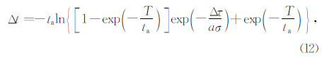
同正向应力扰动的分析一样,在早期应力加载后模型的演化情况与初始条件为2(0)=1(0)exp(Δτ/aσ),μ2(0)=μ1(0)+Δτ/aσ和θ2(0)=θ1(0)的演化情况是一致的,也就是在演化早期加载,失稳时间的推后量Δt是不变的,不过相比于正向静态应力扰动,负向静态应力扰动会使Ω减小,所以静态应力扰动越大,失稳时间推后量Δt为定值的时间就越长.在图 6b 中,当T/ta远远大于1时,同样有Δt近似为Δt≈|Δτ|/b,不过相对于正向静态应力扰动情况,由于Δτ<0导致exp(-Δτ/aσ)较大,进而使得两条渐进线Δt=|Δτ|/b和Δt=T[exp(-Δτ/aσ)-1]交点的横坐标为t0/Tr=1-|Δτ|/{bTr[exp(-Δτ/aσ)-1]};同样地,通过求导可知随|Δτ|的增大两条渐进线交点会逐渐偏向演化后期,那么就说明随|Δτ|的增大,Dieterich模型(虚线)得到的Δt的变化曲线偏离常数Δt=|Δτ|/b的时间点在逐步推后,这与模拟计算结果(实线)相同(图 6b).在演化的末期,按照Dieterich模型,有Δt≈T[exp(-Δτ/aσ)-1],也就是说t0越接近失稳时刻,Δt就越小.在图 6b中可以看出Δτ=-1 MPa和-2 MPa的模拟计算结果和Dieterich模型所代表的曲线在加载时刻较大时重合且趋于零,不过两者相应的差值却会先增大后减小,最大值达到了Dieterich模型的13%,已表现出与Dieterich模型的差异性了.当τ=-5 MPa,-10 MPa和-15 MPa时,模拟计算结果偏离Dieterich模型所代表的曲线(图 6b,6d),相应的差值可达Dieterich模型的35倍,表明此时Dieterich模型已不再适用,这是因为负向静态应力扰动使得Ω突然减小,而不再满足Dieterich模型的前提条件Ω远远大于1.
b|/|Δτ-/b|=1,其中Δτ+和Δτ-分别为正向和负向静态应力扰动,也就是说时间提前量与时间推后量的比值恒为1.在自加速阶段,根据(12)式并令Δτ+=Δτ,Δτ-=-Δτ,那么有
 | 图 7 绝对值相同的应力扰动对应的失稳时间提前和推后量比值变化图 其中Δta为失稳时间的提前量,Δtd为失稳时间的推后量,t0表示加载时刻,Tr表示模型的演化周期.实线表示模拟计算的结果,虚线是Dieterich模型给出的结果. Fig. 7 Ratio of the time advance and time delay for the same absolute value of static stress perturbation as a function of the triggering time Δta and Δtd represent the time advance and time delay, respectively. The solid and dashed lines show the simulation and calculation derived from the Dieterich model. |
不难看出,(13)式中Δ(Δt)>0即在自加速阶段,对于Dieterich模型有|Δta/Δtd|<1,如图 7中虚线所示,而这与模拟结果(实线)的变化情况基本一致.而Perfettini等(2003)的文章计算出的时间提前量与时间推后量的比值随加载时刻的变化曲线为一震荡曲线,与Dieterich模型和本文的结果均不相同,而且随着t0/Tr的增加,振荡的幅度也在不断增加,远远偏离比值为1.0的情况.
4 讨论在文章中我们使用了1-D弹簧-滑块模型,在这里我们对这个模型做一简单的讨论.首先1-D弹簧-滑块模型等价于空间上滑动和应力均匀分布的断层模型(Rice,1983),它可以用来研究不同情况下断层模型的一阶近似情况(Dieterich,1981),能够突出基本物理特征,进而为我们进一步研究震源机制提供线索.例如,研究者们通过对1-D弹簧-滑块模型的分析认识到存在临界刚度kc,只有当弹簧的刚度系数满足k<kc时,滑块会失稳滑动(Dieterich,1978,1979; Ruina,1983; Gu et al.,1984; Ranjith and Rice,1999).如前所述k与断层尺度l成反比,所以存在最小的断层尺度lc,这一推论表明只有当断层块(fault patch)上的滑动超过临界值时,才会发生失稳滑动,而这就为描述成核过程提供了一种可能的物理模型.又如Bizzarri(2012)利用1-D弹簧-滑块模型来讨论地震循环(earthquake cycle)和循环时间(recurrence time).此外,该1-D弹簧-滑块模型也被用来定性地理解地震触发,像研究动态和静态应力变化的影响(Gomberg et al.,1997; Gomberg et al.,1998; Belardinelli et al.,2003),或者是研究触发机制(Parsons,2005b).其次,1-D弹簧-滑块模型计算简单,有助于我们建立统计模型.像Dieterich(1994)利用1-D弹簧-滑块模型,得到了余震发生率的公式,它可以转化为我们在实际地震数据统计中得到的大森定律(Omori′s law)的形式,进而为该定律中的参数提供相应的物理解释.总而言之,虽然1-D弹簧-滑块模型相对简单,没有考虑断层面的形态、非均匀性和非弹性的影响,但它却能突出断层的基本物理特征,而且计算简单,有助于我们定性理解地震过程,进而指导下一步的研究.
5 结论
本文利用1-D弹簧-滑块模型,并结合R-S摩擦定律,然后利用四阶龙格库塔算法(4th-order Runga-Kutta algorithm)计算得到了不同静态应力扰动下失稳时间的提前和推后量Δt并与Coulomb模型以及Dieterich模型的估计值进行了比较.模拟计算显示,对于R-S摩擦定律,失稳时间提前和推后量的大小与静态应力扰动的大小和作用时间有关,而且正、负向静态应力扰动所对应的情况并不完全一致,这说明有必要分别对两种情况进行研究.具体而言,在震后松弛/滑移阶段和闭锁阶段(<10-10m·s-1)的任意时间加载,断层失稳时间的提前和推后量Δt为定值,其大小随静态应力扰动Δτ绝对值的增大而增大,且正、负向静态应力扰动对应的Δt基本一致,与Dieterich模型的描述相符合.在加速阶段,对于正向静态应力扰动(Δτ>0)和负向静态应力扰动(Δτ<0)绝对值较小的情况,随加载时刻推后失稳时间的变化量Δt将逐渐变小,与Dieterich模型相符,而当Δτ<0且静态应力扰动Δτ绝对值较大时,随加载时刻推后失稳时间的变化量Δt并不会减小,不符合Dieterich模型的描述,反而会增大甚至存在突跳现象.这表明对于描述负向静态应力加载,Dieterich模型并不一定合适,需要判断相应的近似条件Ω>>1是否满足.不过,Dieterich模型得到的绝对值相同静态应力扰动的失稳时间提前量与推后量比值变化情况却与模拟计算值基本一致,即Dieterich模型可以反映出正、负向静态应力扰动下失稳时间提前量变化与推后量变化的差异性.总体上看,Dieterich模型可以很好地描述1-D断层受静态应力扰动后失稳时间提前和推后量的变化情况.
对于Coulomb模型,它假定在震后松弛/滑移阶段和闭锁阶段,断层的滑移速率为零(Perfettini et al.,2003),这与R-S摩擦定律在震后松弛/滑移阶段和闭锁阶段的情况近似(<10-10m·s-1),所以计算结果显示在震后松弛/滑移阶段和闭锁阶段R-S摩擦定律和Coulomb定律给出的结果是一致的.对于正向静态应力扰动,二者相符的时间随静态应力扰动绝对值的增大,从80%的演化周期减少至50%,而对负向静态应力扰动则从85%增大至95%.当模型演化至加速阶段时,速率变大,相应的扰动后失稳时间变化量就与Coulomb模型存在较大差异.此外,时间提前量与推后量的比值结果更与Coulomb模型的推论相异.这些结果都表明与R-S摩擦定律或Dieterich模型相比,Coulomb模型不能完整地给出受到静态剪应力扰动后断层失稳时间提前或推后的估计值,也无法反映出正、负向静态应力扰动下失稳时间提前量变化与推后量变化的差异性.
| [1] | Barbot S, Lapusta N, Avouac J-P. 2012. Under the hood of the earthquake machine:Toward predictive modeling of the seismic cycle. Science, 336(6082):707-710. |
| [2] | Belardinelli M E, Bizzarri A, Cocco M. 2003. Earthquake triggering by static and dynamic stress changes. Journal of Geophysical Research, 108(B3):2135, doi:10.1029/2002JB001779. |
| [3] | Bhattacharya P, Rubin A M. 2014. Frictional response to velocity steps and 1-D fault nucleation under a state evolution law with stressing-rate dependence. Journal of Geophysical Research:Solid Earth, 119(3):2272-2304. |
| [4] | Bizzarri A. 2012. What can physical source models tell us about the recurrence time of earthquakes?. Earth-Science Reviews, 115(4):304-318. |
| [5] | Dieterich J H. 1978. Time-dependent friction and the mechanics of stick-slip. Pure and Applied Geophysics, 116(4):790-806. |
| [6] | Dieterich J H. 1979. Modeling of rock friction:1. Experimental results and constitutive equations. Journal of Geophysical Research, 84(B5):2161-2168. |
| [7] | Dieterich J H. 1981. Constitutive properties of faults with simulated gouge.//Mechanical Behavior of Crustal Rocks. American Geophysical Union:103-120. |
| [8] | Dieterich J H. 1992. Earthquake nucleation on faults with rate- and state-dependent strength. Tectonophysics, 211(1-4):115-134. |
| [9] | Dieterich J H. 1994. A constitutive law for rate of earthquake production and its application to earthquake clustering. Journal of Geophysical Research, 99(B2):2601-2618. |
| [10] | Freed A M. 2005. Earthquake Triggering by static, dynamic, and postseismic stress transfer. Annual Review of Earth and Planetary Sciences, 33(1):335-367. |
| [11] | Gomberg J, Blanpied M L, Beeler N M. 1997. Transient triggering of near and distant earthquakes. Bulletin of the Seismological Society of America, 87(2):294-309. |
| [12] | Gomberg J, Beeler N M, Blanpied M L et al. 1998. Earthquake triggering by transient and static deformation. Journal of Geophysical Research, 103(B10):24411-24426. |
| [13] | Gomberg J, Beeler N, Blanpied M. 2000. On rate-state and Coulomb failure models. Journal of Geophysical Research, 105(B4):7857-7871. |
| [14] | Gomberg J, Reasenberg P, Cocco M, et al. 2005a. A frictional population model of seismicity rate change. Journal of Geophysical Research, 110(B5):B05S03, doi:10.1029/2004JB003404. |
| [15] | Gomberg J, Belardinelli M, Cocco M, et al. 2005b. Time-dependent earthquake probabilities. Journal of Geophysical Research, 110(B5):B05S04 doi:10.1029/2004JB003405. |
| [16] | Gu J-C, Rice J R, Ruina A L, et al. 1984. Slip motion and stability of a single degree of freedom elastic system with rate and state dependent friction. Journal of the Mechanics and Physics of Solids, 32(3):167-196. |
| [17] | Hardebeck J L. 2004. Stress triggering and earthquake probability estimates. Journal of Geophysical Research, 109(B4):B04310, doi:10.1029/2003JB002437. |
| [18] | Harris R A, Simpson R W. 1992. Changes in static stress on southern California faults after the 1992 Landers earthquake. Nature, 360(6401):251-254. |
| [19] | Harris R A, Simpson R W. 1998. Suppression of large earthquakes by stress shadows:A comparison of Coulomb and rate- and-state failure. Journal of Geophysical Research, 103(B10):24439-24451. |
| [20] | Kame N, Fujita S, Nakatani M, et al. 2013a. Effects of a revised rate- and state-dependent friction law on aftershock triggering model. Tectonophysics, 600:187-195. |
| [21] | Kame N, Fujita S, Nakatani M, et al. 2013b. Earthquake cycle simulation with a revised rate- and state-dependent friction law. Tectonophysics, 600:196-204. |
| [22] | Kaneko Y, Lapusta N. 2008. Variability of earthquake nucleation in continuum models of rate- and-state faults and implications for aftershock rates. Journal of Geophysical Research, 113(B12):B12312, doi:10.1029/2007JB005154. |
| [23] | Kaneko Y, Avouac J-P, Lapusta N. 2010. Towards inferring earthquake patterns from geodetic observations of interseismic coupling. Nature Geoscience, 3(5):363-369. |
| [24] | King G C P, Stein R S, Lin J. 1994. Static stress changes and the triggering of earthquakes. Bulletin of the Seismological Society of America, 84(3):935-953. |
| [25] | King G C P, Cocco M. 2001. Fault interaction by elastic stress changes:New clues from earthquake sequences. Advances in Geophysics, 44:1-38, 1-VIII. |
| [26] | Marone C. 1998. Laboratory-derived friction laws and their application to seismic faulting. Annual Review of Earth and Planetary Sciences, 26(1):643-696. |
| [27] | Parsons T, Toda S, Stein R S, et al. 2000. Heightened odds of large earthquakes near Istanbul:an interaction-based probability calculation. Science, 288(5466):661-665. |
| [28] | Parsons T. 2005a. Significance of stress transfer in time-dependent earthquake probability calculations. Journal of Geophysical Research, 110(B5):B05S02, doi:10.1029/2004JB003190. |
| [29] | Parsons T. 2005b. A hypothesis for delayed dynamic earthquake triggering. Geophysical Research Letters, 32:L04302, doi:10.1029/2004GL021811. |
| [30] | Perfettini H, Schmittbuhl J, Cochard A. 2003. Shear and normal load perturbations on a two-dimensional continuous fault:1. Static triggering. Journal of Geophysical Research, 108(B9):2408, doi:10.1029/2002JB001804. |
| [31] | Perfettini H, Avouac J-P. 2004a. Postseismic relaxation driven by brittle creep:A possible mechanism to reconcile geodetic measurements and the decay rate of aftershocks, application to the Chi-Chi earthquake, Taiwan. Journal of Geophysical Research, 109(B2):B02304, doi:10.1029/2003JB002488. |
| [32] | Perfettini H, Avouac J P. 2004b. Stress transfer and strain rate variations during the seismic cycle. Journal of Geophysical Research, 109(B6):B06402, doi:10.1029/2003JB002917. |
| [33] | Ranjith K, Rice J R. 1999. Stability of quasi-static slip in a single degree of freedom elastic system with rate and state dependent friction. Journal of the Mechanics and Physics of Solids, 47(6):1207-1218. |
| [34] | Rice J R. 1983. Constitutive Relations for Fault Slip and Earthquake Instabilities. Pure and Applied Geophysics, 121(3):443-475. |
| [35] | Rubin A M, Ampuero J-P. 2005. Earthquake nucleation on (aging) rate and state faults. Journal of Geophysical Research, 110(B11):B11312, doi:10.1029/2005JB003686. |
| [36] | Ruina A. 1983. Slip instability and state variable friction Laws. Journal of Geophysical Research, 88(B12):10359-10370. |
| [37] | Scholz C H. 1998. Earthquakes and friction laws. Nature, 391(6662):37-42. |
| [38] | Segall P. 2010. Earthquake and Volcano Deformation. Princeton:Princeton University Press. |
| [39] | Stein R S, Barka A A, Dieterich J H. 1997. Progressive failure on the North Anatolian fault since 1939 by earthquake stress triggering. Geophysical Journal International, 128(3):594-604. |
| [40] | Stein R S. 1999. The role of stress transfer in earthquake occurrence. Nature, 402(6762):605-609. |
| [41] | Stein S, Wysession M. 2003. An Introduction to Seismology, Earthquakes, and Earth Structure. Malden:Blackwell Publishing. |