 2015, Vol. 58


2. 甘肃省地震局, 兰州 730000
2. Earthquake Administration of Gansu Province, Lanzhou 730000, China
First we used the high frequency envelope difference of the three components with continuous waveforms of the station MXT to detect missing earthquakes in the three hours after the mainshock. In order to suppress low frequency interference, the waveforms were filtered by a 15 Hz high pass forth-order zero phase Butterworth filter. We calculated the difference of maxima envelope and minimum envelope using three-component added waveforms, and then picked out the clear "double peaks" by hand in the high frequency envelope difference as the detected missing earthquakes. The magnitude of missing earthquakes was determined by linear transformation of envelope peak values, whose transformation parameters were calculated using the envelope peak values and magnitude of aftershocks in the catalog. Second, we used the modified Omori's law to fit seismic frequency and seismic moment of the new catalog with added earthquakes detected. Temporal decay characteristics were analyzed by comparing the decay parameter p in different fitting methods and different aftershock sequences.
By the detection we found 139 missing earthquakes in the three hours after the mainshock, of which the largest is ML3.6, and about 6 times missing earthquakes in 1000 seconds after the mainshock more than that in the original catalog. The estimation result of p value is about 1.07, which shows that the temporal decay rate of the Minxian-Zhangxian earthquake is similar to the average rate of other worldwide earthquakes. The decay rate may be under estimated if the missing earthquakes are not added to the catalog. By direct obtaining the seismicity rate curve from high frequency envelope difference and fitting the curve using three kinds of decay modes, we did not observe the phenomenon of early aftershock deficiency in the aftershock sequence.
We note that the accuracy and precision of the result of aftershock sequence temporal decay analysis can be improved by adding missing earthquakes to the catalog. If there is no missing earthquake detected, it is better to use seismic moment to estimate the temporal decay parameters of the aftershock sequence and give full consideration of the precision. It is important to choose appropriate fitting methods according to catalog completeness in aftershock decay analysis.
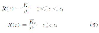
中强地震后往往发生大量余震,余震序列衰减特征研究是震后趋势判断、强余震预测和发震构造分析等研究的组成部分,对理解主震发震过程、地震危险性分析和抗震救灾有重要作用.研究余震序列随时间的衰减特征多采用具有一定物理背景的统计模型,包括修正的大森公式(Utzu et al.,1961;1995)、ETAS模型(Ogata,1988;1989;2001;蒋海昆等,2007)以及BASS模型(Sheherbakov and Turcotle.,2004;Turcotte et al.,2007)等.其中修正的大森公式是对余震序列衰减较为简便的描述方式,表达式为

其中n(t)为单位时间内余震的频度,K、p、c为常数.K与主震震级和统计所选择的震级下限有关.p表示余震序列衰减快慢,全球许多中强地震余震序列计算结果显示p值接近于1(Utzu et al.,1995;Rabinnovitz and Steinberg,1998;Lolli and Gasperini,2003;Husen et al.,2004;Gentili et al.,2008;赵志新等,1992),而与所选择的震级下限无关.c是小正数,使得表达式分母不为0(宋金和蒋海昆,2009).
利用修正的大森公式对余震序列衰减特征进行研究多基于地震目录.随着测震台网数字化连续波形资料的积累,利用高频段连续波形记录拾取地震目录遗漏的余震,成为深入研究中强地震早期余震特征的有效手段(Peng et al.,2006;2007;Peng and Zhao,2009;Enescu et al.,2007;2009;Lengline et al.,2012;Marsan and Enescu.,2012;Sawazaki and Enescu,2014;Kato and Obara,2014).研究结果显示,主震后数分钟到数小时内目录往往遗漏较多的地震.加入这些遗漏地震有助于更加精确地测定p值、c值等余震衰减参数(Enescu et al.,2007),为研究余震的触发机制、主震破裂与余震发生的关系以及发震断层的物理性质提供了重要的参考资料.
2013年7月22日7点45分56.2秒在甘肃省定西市岷县、漳县交界发生MS6.6地震.此次地震发生在南北地震带中北段,构造较为复杂的甘东南地区(郑文俊等,2013;孙蒙等,2015),历史上地震活动较为活跃(国家地震局震害防御司,1995).本文首先使用距离余震区最近的岷县台(MXT)(如图 1所示)高频段连续记录波形,检测主震发震后3 h内目录遗漏的地震,再基于修正的大森公式分析岷县漳县地震余震序列时域衰减特征.
 | 图 1 地震岷县漳县地震余震序列震中位置与观测台站分布图 灰色五角星为主震震中位置,空心圆圈为余震震中位置, 三角形为甘肃台网台站,灰色曲线为区域主要断层.Fig. 1 Epicenter and station distribution of Minxian-Zhangxian earthquake aftershock sequence The gray star represents the epicenter of mainshock, circles represent epicenters of aftershocks, triangles represent stations of Gansu seismic network, and the gray lines represent main faults. |
大震发生后地震目录往往会遗漏较多的余震事件(Enescu et al.,2007;Peng and Zhao,2009;Lengline et al.,2012),造成余震遗漏的主要原因在于主震及较大余震的面波等后续震相及尾波的干扰,其中所含低频成分较多(Peng et al.,2006).为了抑制低频干扰的影响,本研究使用4阶零相移Butterworth滤波器对连续波形进行截止频率为15 Hz的高通滤波,对三分向高频波形求和,再计算极大值与极小值包络之差的对数(本文简称为高频包络差).图 2为岷县台(MXT)、临潭台(LTT)、迭部台(DBT)、合作台(HZT)、武都台(WDT)和静宁台(JNT)6个记录信噪比较高且连续性较好的台站主震后1000 s内归一化高频包络差.距离主震震中最近的岷县台记录地震信号的信噪比最高,本文仅使用岷县台的数据检测目录遗漏的地震.
 | 图 2 六个台站归一化高频包络差计算结果对比图 黑色波形为归一化包络差计算结果,右侧标注了台站名和距主震震中的距离; 灰色实线为目录中的地震事件,灰色虚线为目录中给出的单台记录地震事件.Fig. 2 Comparison of normalized high frequency envelope difference of 6 stations The black waveforms are high frequency envelope difference results, station name and epicenter distance of mainshock are marked on the right. The gray lines represent earthquakes in the catalog, and the dashed lines represent single station events in the catalog. |
Peng等(2007)通过研究日本多个地震,认为以1.5级为界包络振幅对应的震级与台网测量震级间存在两组线性关系.Wang等(2011)也发现经过滤波后的地震波振幅与震级存在线性关系.鉴于岷县台BBVS-60地震计在15~50 Hz频段仪器响应放大倍数近似为常数,其仪器响应亦近似为线性.因而可设高频包络差与震级存在与Peng等(2007)形式类似的线性关系:
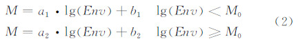
其中M为震级,Env为高频包络差峰值振幅,M0为不同线性关系的分界震级.
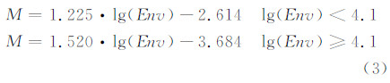
采用与Marsan和Enescu(2012)类似的方法,利用目录已有地震的震级与包络尖峰值的对应关系,确定线性变换参数.使用《甘肃省测震台网地震观测报告》给出的余震目录,并根据多台波形互相关震相检测震级估计结果1),对其中主震后的第一个余震和部分单台记录地震事件的震级进行了修正.通过主震后3 h内目录给出的164个地震线性拟合求取式(2)中的参数a1、b1、a2、b2和M0.如图 3所示,估计震级以ML4.1为界,包络差峰值振幅通过两组线性关系拟合到目录给出的震级.式(3)给出了计算得到的线性拟合关系式.
1)谭毅培,陈继锋,曹井泉等.2013年甘肃岷县漳县6.6级地震余震序列目录完备性研究:基于对单台记录地震事件震中与震级的估计.地震学报,录用待刊.
 | 图 3 包络差峰值振幅与目录给出震级线性拟合结果图 横坐标为利用包络差振幅对数估计得到的震级,纵坐标为目录给出的震级.黑色圆圈为未经线性变换震级校正的结果,灰色圆圈为经过线性变换震级校正的结果.Fig. 3 Linear fitting result of high frequency envelope difference amplitude and magnitude in the catalog X-axis is calculated magnitude from high frequency envelope difference in log, Y-axis is magnitude in the catalog. The black circles represent uncorrected results, and the gray circles represent corrected results by linear transformation. |
包络差峰值振幅经过式(3)线性变换后所得震级估计值与目录给出震级的误差分布如图 4所示.误差标准差为0.2357,与区域测震台网地震编目震级误差水平0.2接近,因而经线性变换的包络峰值振幅可以较好地拟合目录已有地震的震级,即利用其拾取目录遗漏地震所得震级是基本可靠的.
 | 图 4 主震后3 h内164个地震高频包络差方法估计震级与目录给出震级误差统计分布图Fig. 4 Error distribution of magnitude calculated from high frequency envelope difference with linear transformation minus magnitude in the catalog of 164 earthquake events in 3 hours after the mainshock |
使用与Peng等(2006)相同的方法检测拾取目录遗漏的地震,即人工挑选高频包络差中较为清晰的双脉冲(Double peaks)作为检测到的遗漏地震.双脉冲中振幅较大的峰值作为遗漏地震的震级,双脉冲中点作为发震时刻.如图 5所示,通过上述方法在主震后3 h内共检测到目录遗漏的ML1.0以上地震139个,其中在主震后1000 s内检测到ML1.0以上遗漏地震67个,约为目录给出余震数量的6倍.图 5中同时画出了目录给出的11个地震,其发震时刻与包络差双脉冲位置亦吻合较好.
 | 图 5 主震后1000 s内检测到的目录遗漏地震 (a) 主震发生到主震后500 s结果; (b) 主震后500~1000 s的结果.灰色圆圈为检测到的遗漏地震, 五角星为主震,三角形为目录给出的地震事件,其上标注了目录给出的震级.Fig. 5 Missing earthquakes detected in 1000 seconds after the mainshock (a) Detection result of 500 seconds and (b) 500~1000 seconds after the mainshock. The gray circles represent detected earthquake events, the star represents the mainshock, and the triangles represent events in the catalog whose magnitude is marked on the top. |
本节基于修正的大森公式,拟合衰减参数,分析岷县漳县地震余震序列时域衰减特征.首先利用式(1)拟合余震频度随时间的衰减.蒋长胜等(2013)通过尝试不同震级下限对岷县漳县地震余震序列早期特征分析的影响,认为震级下限MC取ML1.0或ML1.1时拟合程度最佳.利用“震级-序号法”(Huang,2006;Jia et al.,2012;2014;蒋长胜和吴忠良,2011,蒋长胜等,2013)对补充遗漏地震后余震目录的分析结果(图 6)显示,在ML=1.0时地震累计数量最多.综合以上分析,本文余震数目统计震级下限取ML1.0.参考Peng等(2006)工作,统计窗长为时间轴对数坐标下0.2,并以对数坐标下0.2滑动,余震频度为单位窗内余震的个数除以时间线性坐标轴下的窗长.统计的起点设为10-3天,约为86.4 s,是考虑到拾取的第一个遗漏地震发震时刻约为主震后61 s,之前高频包络差能量主要由主震所贡献.
 | 图 6 余震目录“震级-序号法”分析结果图 (a) 余震震级随序号的变化,红色圆点为本文检测到的遗漏地震,黑色圆点为目录给出的地震;(b) 地震累计数量随震级的变化.Fig. 6 “Magnitude sequential number method” analysis result of aftershock sequence (a) Plots of magnitudes versus the sequential numbers. The red dots represent detected events and the black dots represent earthquake events in the catalog. (b) Cumulative number of earthquakes versus magnitude. |
Kagan和Houston(2005)发现余震地震矩随时间衰减也符合类似修正的大森公式的关系,并提出分析地震矩随时间的衰减可以降低目录遗漏地震对拟合参数的影响.本文同样使用式(1)拟合地震矩随时间的衰减,震级下限和统计窗长设置与余震频度拟合相同.由于震级较小的余震没有可靠的距张量反演结果,使用陈继锋和杨立明(2011)得到的甘肃地区地震矩与区域震级的统计关系:

其统计样本为ML2.0~6.0的中小地震,岷县漳县地震最大余震为ML5.7,而小于ML2.0的余震地震矩较小,其误差对分析地震矩衰减的影响亦较小,因而此统计关系基本适合本研究的需要.
图 7和图 8分别给出了余震频度和余震地震矩衰减的参数拟合结果.对比加入遗漏地震与未加入遗漏地震拟合的结果可以发现如下特征:
 | 图 7 余震频度随时间衰减参数拟合结果 圆圈表示未加入遗漏地震的结果,灰色虚线为其拟合曲线;十叉表示加入遗漏地震的结果,灰色实线为其拟合曲线,图中标注了拟合参数值.Fig. 7 Parameter fitting results of temporal decay rate of aftershocks with modified Omori′s law for catalog events (cross) and catalog+detected events (circle) The gray curve and dashed curve are fitting results of catalog+detected events and catalog events respectively. Fitting parameters are written in the figure. |
 | 图 8 地震矩随时间衰减参数拟合结果 图注同图7.Fig. 8 Parameter fitting results of temporal decay of moment release with modified Omori′s law Others are same as Fig.7. |
1)余震频度和地震矩拟合所得p值在加入遗漏地震后都出现增大,c值减小,而K值基本保持不变.在Enescu等(2007;2009)对日本5个地震序列的研究中,有4个也出现了加入遗漏地震后p值上升的情况,可见早期余震序列目录遗漏地震很可能使得序列衰减速率出现低估.
2)在加入遗漏地震后,余震频度和地震矩拟合所得p值都为1.07,与Utzu等(1995)对全球200余个地震序列分析得到的平均值p=1.1接近,因此认为岷县漳县地震余震序列衰减速率处于全球平均水平.
对比余震频度和地震矩两种方式所得参数拟合结果,存在如下特征:
1)余震频度拟合参数的置信区间更小,即参数估计的精度更高;
2)余震频度拟合p值和c值在加入遗漏地震后变化幅度更大,似乎能够印证Kagan和Houston(2005)提出的“遗漏地震对地震矩随时间特征衰减影响更小”的结论;
3)地震矩拟合所得c值远小于余震频度拟合结果.
加入遗漏地震后,两种拟合方法得到p值都为1.07,而未加入遗漏地震地震矩拟合得到p值为1.04,更接近1.07.综合考虑参数估计的准确度和精度,在分析余震序列衰减速率时,加入遗漏地震拾取的余震频度拟合可以得到较好的结果;若使用未加入遗漏地震的目录,则地震矩拟合得到的结果更为准确,但要充分考虑到其精度误差.
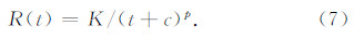
3.2 早期余震缺失判别Peng等(2006)通过直接使用高频包络计算地震频度,发现2004年Parkfield地震主震破裂与余震序列衰减过程之间存在一个余震频度基本保持稳定的时间段,作者称之为早期余震缺失(Early Aftershock Deficiency,EAD).本节使用相似的方法直接通过高频包络差计算地震频度曲线,并使用三种衰减模式拟合地震频度曲线,探讨岷县漳县地震主震后是否存在类似的早期余震缺失现象.
地震频度从岷县台P波到达时刻算起,窗长为时间轴对数坐标下0.2,并以对数坐标下0.01滑动.三种衰减模式分别为直线衰减:

采用赤池信息准则(Akaike,1974)作为三种模式拟合效果比较的标准:

图 9展示了三种模式拟合程度的比较结果,直线衰减和修正的大森公式衰减AIC值为常数,两段线衰减模式的AIC值为t0的函数.其中两段线衰减模式的AIC值在t0=14.13 s时取得最小值,在前30 s内两段线模式AIC值最小,30 s后修正的大森公式衰减模式AIC值成为最小值.第2节中检测到的第一个余震约为主震后61 s,主震后30 s内间内高频包络差能量主要由主震贡献,余震的能量湮没在主震后续震相能量中无法分辨,无法证明在此时间段内余震存在缺失,因而未发现岷县漳县地震主震后存在早期余震缺失现象.
 | 图 9 使用三种模式对基于高频包络差计算的地震频度曲线拟合的比较结果 (a) AIC值比较; (b) 三种模式拟合结果,并标明了拟合参数值.其中绿色为两段线衰减模式,蓝色为直线衰减模式,红色为修正的大森公式衰减模式.黑色虚线为两段线衰减模式AIC取得最小值的时间点,距岷县台主震P波到时14.13 s.Fig. 9 Comparison result of fitting for seismic rate curve calculated from high frequency envelope difference using three kinds of decay model (a) Comparison of AIC value; (b) Fitting results and parameters of three model. The green represents broken line decay model, the blue represents linear decay model and the red represents modified Omori′s law decay model. The x-axis of black dashed line is the time that AIC of broken line decay model get the minimum value, which is 14.13 s after the P arriving time of mainshock on MXT. |
本文使用岷县台高频包络差检测目录遗漏的地震,并基于修正的大森公式分析了岷县漳县地震余震序列时域衰减特征.通过检测在主震后3 h内共拾取到目录遗漏的ML1.0以上地震139个,其中主震后1000 s内检测到遗漏地震数量约为目录给出余震数量的6倍.遗漏地震参与分析对于估计余震序列衰减特征有重要作用,通过余震频度拟合和地震矩拟合得到的余震衰减速率p值皆为1.07,表明岷县漳县地震余震序列衰减速率与全球平均水平接近.在分析余震序列衰减速率时,加入遗漏地震并利用频度拟合所得结果较优;若无条件拾取目录遗漏地震,则使用地震矩拟合得到的结果更为准确,但需充分考虑其误差.三种衰减模式拟合直接使用高频包络差计算地震频度曲线比较结果显示,无法证明岷县漳县地震主震后存在早期余震缺失现象.
高频包络差方法一个显著的优势在于有较高的计算效率,适用于震后快速趋势判断和强余震预测等对计算时间要求较高的研究.与匹配滤波技术(Shally et al.,2007;Peng and Zhao,2009)等模板识别类方法相比,本文方法仅使用一个台站的连续波形记录,无需选择地震模板以及波形互相关计算,计算过程简单快捷、可以在主震发生后快速给出遗漏地震检测结果.同时不可否认,利用高频包络差检测目录遗漏地震需要人工手动拾取,使得结果不可避免带有一定主观性,且无法得到遗漏地震震中估计结果.对于余震序列时空变化的研究、利用遗漏地震作为补充对发震构造进行分析等研究方向,需选用模板识别类方法检测目录遗漏的地震.
本文研究表明目录完整性对余震序列衰减参数估计结果有一定的影响,早期余震缺失可能使得p值估计结果偏低,而c值估计结果偏高.在分析余震序列衰减特征的实际研究工作中,需根据地震目录完整性选择适当的拟合方法.当然,仅凭对岷县漳县地震余震序列结果无法确定遗漏地震检测对衰减特征分析的作用,需要今后对更多的中强地震余震序列进行分析研究.
使用三种模式对直接使用高频包络差计算的地震频度曲线拟合p值(0.71~0.76)均小于余震频度衰减和地震矩衰减拟合结果(1.07),Peng等(2006)拟合余震频度曲线的p值也小于利用地震目录的拟合值,表明直接使用高频包络计算地震频度曲线无法用来分析余震序列的衰减速率.
本文研究结果展示了在我国西部固定台网较稀疏的地区,利用高频波形拾取遗漏地震,进而更加精确测定余震序列衰减速率研究的可行性.由于地震波高频成分随震中距增大能量衰减较快,因而利用波形高频成分拾取目录遗漏地震需要震中距较小台站的波形记录.前人研究区域多在美国加州、土耳其和日本等台网密度较大的地区(Peng et al.,2006;2007;Enescu et al.,2007;2009;Bouchon et al.,2011;Lengline et al.,2012;Marsan et al.,2012;Kato et al.,2012;Kato and Obara,2014;Wu et al.,2014),有较多距离余震区近的台站,如Peng等(2006)对2004年Parkfield地震研究中有15个震中距小于30 km的台站可供选择,而本文研究对象岷县漳县地震只有岷县台震中距小于30 km.现阶段我国区域测震台网在中强地震后架设流动台需要数小时时间,因而固定台站记录在多数情况下是检测早期余震序列目录遗漏地震的唯一地震波形资料.随着我国测震台网基础建设的不断发展,包括中强地震余震序列衰减特征分析在内的地震学研究亦将不断深入.
致 谢 感谢审稿专家宝贵的建设性意见,感谢中国地震局张浪平博士、甘肃省地震局张元生研究员、中国地震局地球物理研究所蒋长胜研究员和韩立波博士的指导和建议.本文部分图件采用GMT软件包绘图.| [1] | Akaike H. 1974. A new look at the statistical model identification. IEEE Trans. Autom. Control, 19(6): 716-723. |
| [2] | Bouchon M, Karabulut H, Aktar M, et al. 2011. Extended nucleation of the 1999 MW7.6 Izmit earthquake. Science, 331(6019): 877-810. |
| [3] | Chen J F, Yang L M. 2011. Study of source parameters′ relationship in Gansu province. Seismological and Geomagnetic Observation and Research (in Chinese), 32(1): 10-14. |
| [4] | Disaster Prevention Department of China Earthquake Administration. 1995. China historical earthquake catalog (23rd century BC—1911 AD) (in Chinese). Beijing: Seismological Press, 497-499. |
| [5] | Enescu B, Mori J, Miyazawa M. 2007. Quantifying early aftershock activity of the 2004 mid-Niigata Prefecture earthquake (Mw6.6). J. Geophys. Res., 112: B04310, doi: 10. 1029/2006JB004629. |
| [6] | Enescu B, Mori J, Miyazawa M, et al. 2009. Omori-Utsu law c-values associated with recent moderate earthquakes in Japan. Bull. Seism. Soc. Am., 99(2A): 884-891. |
| [7] | Gentili S, Bressan G. 2008. The partitioning of radiated energy and the largest aftershock of seismic sequences occurred in the northeastern Italy and western Slovenia. J. Seismol., 12(3): 343-354. |
| [8] | Huang Q H. 2006. Search for reliable precursors: A case study of the seismic quiescence of the 2000 western Tottori prefecture earthquake. J. Geophys. Res., 111(B4): B04301, doi: 10.1029/2005/JB003982. |
| [9] | Husen S, Wiemer S, Smith R B. 2004. Remotely triggered seismicity in the Yellowstone National Park region by the 2002 Mw7.9 Denali Fault earthquake, Alaska. Bull. Seism. Soc. Am., 94(6B): S317-S331. |
| [10] | Jia K, Zhou S, Wang R. 2012. Stress interactions within the strong earthquake sequence from 2001 to 2010 in the Bayankala block of eastern Tibet. Bull. Seism. Soc. Am., 102(5): 2157-2164. |
| [11] | Jia K, Zhou S Y, Zhuang J C, et al. 2014. Possibility of the independence between the 2013 Lushan earthquake and the 2008 Wenchuan earthquake on Longmen Shan fault, Sichuan, China. Seismological Research Letters, 85(1): 60-67, doi: 10.1785/0220130115. |
| [12] | Jiang C S, Wu Z L. 2011. Intermediate-term medium-range accelerating moment release (AMR) prior to the 2010 Yushu MS7.1 earthquake. Chinese J. Geophys. (in Chinese), 54(6): 1501-1510, doi: 10.3969/j.issn.0001-5733.2011.06.009 . |
| [13] | Jiang C S, Wu Z L, Han L B, et al. 2013. Effect of cutoff magnitude Mc of earthquake catalogues on the early estimation of earthquake sequence parameters with implication for the probabilistic forecast of aftershocks: the 2013 Minxian-Zhangxian, Gansu, MS6.6 earthquake sequence. Chinese J. Geophys. (in Chinese), 56(12): 4048-4057, doi: 10.6038/cjg20131210. |
| [14] | Jiang H K, Zheng J C, Wu Q, et a1. 2007. Earlier statistical features of ETAS model parameters and their seismological meanings. Chinese J. Geophys. (in Chinese), 50(6): 1778-1786. |
| [15] | Kagan Y Y, Houston H. 2005. Relation between mainshock rupture process and Omori′s law for aftershock moment release rate. Geophys. J. Int., 163(3): 1039-1048. |
| [16] | Kato A, Obara K, Igarasgi T, et al. 2012. Propagation of slow slip leading up to the 2011 MW9.0 Tohoku-Oki earthquake. Science, 335(6069): 705-708. |
| [17] | Kato A, Obara K. 2014. Step-like migration of early aftershocks following the 2007 MW6.7 Noto-Hanto earthquake, Japan. Geophys. Res. Lett., 41(11): 3864-3869, doi: 10.1002/2014GL060427. |
| [18] | Lengliné O, Enescu B, Peng Z X, et al. 2012. Decay and expansion of the early aftershock activity following the 2011, Mw9.0 Tohoku earthquake. Geophysical Research Letters, 39(18), doi: 10.1029/2012GL052797. |
| [19] | Lolli B, Gasperini P. 2003. Aftershocks hazard in Italy Part I: Estimation of time-magnitude distribution model parameters and computation of probabilities of occurrence. J. Seismol., 7(2): 235-257. |
| [20] | Marsan D, Enescu B. 2012. Modeling the foreshock sequence prior to the 2011, MW9.0 Tohoku, Japan, earthquake. J. Geophys. Res., 117: B06316, doi: 10.1029/2011JB009039. |
| [21] | Ogata Y. 1988. Statistical models for earthquake occurrences and residual analysis for point processes. J. Amer. Statist. Assoc., 83(401): 9-27. |
| [22] | Ogata Y. 1989. Statistical model for standard seismicity and detection of anomalies by residual analysis. Tectonophysics, 169(1-3): 159-174. |
| [23] | Ogata Y. 2001. Increased probability of large earthquakes near aftershock regions with relative quiescence. J. Geophys. Res., 106(B5): 8729-8744. |
| [24] | Peng Z G, Vidale J E, Houston H. 2006. Anomalous early aftershock decay rate of the 2004 Mw6.0 Parkfield, California, earthquake. Geophys. Res. Lett., 33(17): L17307, doi: 10.1029/2006GL026744. |
| [25] | Peng Z G, Vidale J E, Ishii M, et al. 2007. Seismicity rate immediately before and after main shock rupture from high-frequency waveforms in Japan. J. Geophys. Res., 112: B03306, doi: 10.1029/2006JB004386. |
| [26] | Peng Z G, Zhao P. 2009. Migration of early aftershocks following the 2004 Parkfield earthquake. Nature Geoscience, 2(12): 877-881. |
| [27] | Rabinowitz N, Steinberg D M. 1998. Aftershock decay of three recent strong earthquakes in the Levant. Bull. Seism. Soc. Am., 88(6): 1580-1587. |
| [28] | Sawazaki K, Enescu B. 2014. Imaging the high-frequency energy radiation process of a main shock and its early aftershock sequence: The case of the 2008 Iwate-Miyagi Nairiku earthquake, Japan. J. Geophys. Res.: Solid Earth, 119(6): 4729-4746, doi: 10.1002/2013JB010539. |
| [29] | Shally D R, Beroza G C, Ide S. 2007. Non-volcanic tremor and low-frequency earthquake swarms. Nature, 446(7133): 305-307. |
| [30] | Sheherbakov R, Turcotte D L. 2004. A modified form of Bath′s Law. Bull. Seism. Soc. Am., 94(5): 1968-1975. |
| [31] | Song J, Jiang H K. 2009. A review on decay and generation of aftershock activity. Seismology and Geology (in Chinese), 31(3): 559-571. |
| [32] | Sun M, Wang W M, Wwang X et al .2015.Rupture process of the Minxian-Zhangxian, Gansu, China MS6.6 earthquake on 22 July 2013.Chinese J. Geophys. (in Chinese),58(6): 1909-1918,doi: 10.6038/cjg20150607. |
| [33] | Turcotte D L, Holliday J R, Rundle J B. 2007. BASS, an alternative to ETAS. J. Geophys. Res., 34(12): L12303. |
| [34] | Utsu T. 1961. A statistical study on the occurrence of aftershocks. Geophys. Mag., 30: 521-605. |
| [35] | Utsu T, Ogata Y, Matsuura R S. 1995. The centenary of the Omori formula for a decay law of aftershock activity. J.Phys. Earth., 43(1): 1-33. |
| [36] | Wang J, Schweitzer J, Tilmann F, et al. 2011. Application of the multichannel Wiener filter to regional event detection using NORSAR seismic-array data. Bull. Seism. Soc. Am., 101(6): 2887-2896. |
| [37] | Wu C Q, Meng X F, Peng Z G, et al. 2014. Lack of spatiotemporal localization of foreshocks before the 1999 MW7.1 Düzce, Turkey, earthquake. Bull. Seism. Soc. Am., 104(1): 560-566. |
| [38] | Zhao Z X, Kazuo O, Kazuo M, et a1. 1992. P values of continental aftershock activity in China. Acta Seismologica Sinica (in Chinese), 14(1): 9-16. |
| [39] | Zheng W J, Yuan D Y, He W G, et al. 2013. Geometric pattern and active tectonics in Southeastern Gansu province: Discussion on seismogenic mechanism of the Minxian-Zhangxian MS6.6 earthquake on July 22, 2013. Chinese J. Geophys. (in Chinese), 56(12): 4058-4071, doi: 10.6038/cjg20131211. |
| [40] | 陈继锋, 杨立明. 2011. 甘肃地区震源参数的相关性研究. 地震地磁观测与研究, 32(1): 10-14. |
| [41] | 国家地震局震害防御司. 1995. 中国历史强震目录(公元前23世纪—公元1911年). 北京: 地震出版社, 497-499. |
| [42] | 蒋长胜, 吴忠良. 2011. 2010年玉树MS7.1地震前的中长期加速矩释放(AMR)问题. 地球物理学报, 54(6): 1501-1510, doi: 10.3969/j.issn.0001-5733.2011.06.009. |
| [43] | 蒋长胜, 吴忠良, 韩立波等. 2013. 地震序列早期参数估计和余震概率预测中截止震级MC的影响: 以2013年甘肃岷县—漳县6.6级地震为例. 地球物理学报, 56(12): 4048-4057, doi: 10.6038/cjg20131210. |
| [44] | 蒋海昆, 郑建常, 吴琼等. 2007. 传染型余震序列模型震后早期参数特征及其地震学意义. 地球物理学报, 50(6): 1778-1786. |
| [45] | 宋金, 蒋海昆. 2009. 序列衰减与余震激发研究进展及应用成果. 地震地质, 31(3): 559-571. |
| [46] | 孙蒙, 王卫民, 王洵 等 .2015.2013年7月22日甘肃岷县—漳县MS6.6地震震源破裂过程. 地球物理学报,58(6): 1909-1918,doi: 10.6038/cjg20150607. |
| [47] | 赵志新, 尾池和夫, 松村一男等. 1992. 中国大陆性地震的余震活动的P值. 地震学报, 14(1): 9-16. |
| [48] | 郑文俊, 袁道阳, 何文贵等. 2013. 甘肃东南地区构造活动与2013年岷县—漳县MS6.6级地震孕震机制. 地球物理学报, 56(12): 4058-4071, doi: 10.6038/cjg20131211. |