 2015, Vol.58


2.中国石油大学(北京), 油气资源与勘探测国家重点实验室, 北京 102249
2.State Key Laboratory of Petroleum Resources and Prospecting, China University of Petroleum, Beijing 102249, China
Seismic interpolation especially the high dimensional interpolation belongs to large-scale computational problems, thus fast algorithms should be chosen to improve the efficiency of seismic interpolation.Sparse transform methods change the interpolation problem into a sparse optimization based on the assumption that seismic data can be expressed sparsely in some transform domain.POCS method is such a method with high efficiency and robust results.However, this method can not get acceptable results for random noise contained data interpolation.The weighted POCS method is a method for random noise contained data interpolation on the basis of the POCS method.But there is no specific explanation of this method up to now.This paper deduced the weighted POCS method from the iterative thresholding method, we proved that the weighted POCS method is a method for unconstrained optimization, the weighted factor can be seen as the coefficient of the fitting error.However, the original POCS method is aiming at an equality constrained optimization.This is the essential difference between them.Meanwhile, we also proposed an improved POCS method with the same computational complexity as the original POCS method.The improved POCS method can realize interpolation and denoising simultaneously by adjustment of the least thresholds.
In order to test the interpolation and denoising capability of the improved POCS method, four data sets were used to make numerical experiments.The first experiment is a synthetic noiseless data interpolation.The dimension of the synthetic data is 256 ×256 with trace distance 25 m and time sampling rate 4 ms.The original POCS method is chosen as the benchmark.Both the computational efficiency and numerical result are comparable for them.The second data is field data with 115 traces.The trace distance is 25 m and the time sampling rate is 4 ms.This experiment also proved that both of them can get comparable results for noiseless data interpolation.The third example is a noise contained data interpolation.The original POCS method can not get acceptable result no matter how to choose the least thresholds, while the improved POCS method can provide good result by choosing the least thresholds carefully.The fourth example also proved that the original POCS method failed in the noise contained field data interpolation, and the improved POCS method is suitable for noise contained data interpolation.Numerical experiment on first-interpolation-then-denoising proved the rationality and robustness of simultaneous interpolation and denoising.
We deduced the weighted POCS method from the iterative thresholding method, and proved that it is a method for unconstrained optimization, the weighting factor is the coefficient of the fitting error.However, the original POCS method is a method for equality constrained optimization.This is the essential difference between them.We also proposed an improved POCS method to realize simultaneous interpolation and denoising.This method just need to adjust the least thresholds to realize noiseless data and random noise contained data interpolation.The computational effort of the improved POCS method is the same as the original POCS method but with more broad applications.
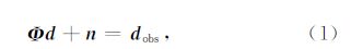
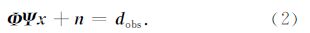
由于采集成本、地形、坏道等因素的限制,野外采集的地震数据经常不满足香农采样定理(陆基孟,1993).不完整的数据会产生采集脚印,严重地影响叠前时间偏移(Symes,2007)、三维表面多次波消除(Berkhout and Verschuur,1997)和全波形反演(Bunks et al.,1995)的效果,因此需要采用插值方法来得到完备的波场信息.地震数据插值不仅能够提供可靠的波场数据,还可以指导采集设计,节约采集成本(Yilmaz,1987).目前,地震插值方法主要包括预测滤波方法(Spitz,1991),基于稀疏变换的方法(Liu and Sacchi,2004;Zwartjes,2005;Herrmann and Hennenfent,2008;Xu et al.,2010),基于波动方程的方法(Ronen,1987;Stolt,2002)和矩阵降秩 方法(Oropeza and Sacchi,2011;Kreimer and Sacchi,2012;Ma,2013). 预测滤波方法专门针对规则不完备采样数据的插值(Spitz,1991);基于波动方程的方法需要地下的参数信息并且计算量较大.随着压缩感知理论引入到图像和三维数据的填充,矩阵/张量完备方法也被用于地震数据插值(Oropeza and Sacchi,2011;Kreimer and Sacchi,2012;Ma,2013),该方法将插值问题看作图像填充问题,基于完整的矩阵或张量的秩最小化来实现地震数据插值.基于稀疏变换的方法利用各种变换,比如 Fourier 变换(Liu and Sacchi,2004;Zwartjes,2005;Xu et al.,2010),Radon 变换(Trad et al.,2002),seislet 变换(Fomel and Liu,2010),Dreamlet变换(耿瑜等,2012),curvelet 变换(Cao et al.,2011;Wang et al.,2011;曹静杰等,2012;Mansour et al.,2013)等作为稀疏变换来压缩地震数据,由于其高效性和稳定性,该方法得到了很大的发展.
野外地震数据经常包含不同类型的噪声,这些噪声可以分为两类:随机噪声和相干噪声.目前的插值方法很少直接研究含噪声数据的插值.对于含随机噪声的采样不足数据,一般是先插值后去噪.Hennenfent和Herrmann(2006)提出了一种基于非规则采样curvelet 变换和阈值法的地震数据插值和去噪;Oropeza和Sacchi(2011)提出了一种同时插值和去噪的重加权替换方法,通过加权来消除随机噪声,Gao等(2013)提出一种加权凸集投影(POCS)方法来同时去噪和插值.
由于地震数据插值需要处理大量数据,因此属于大规模计算问题,需要快速稳定的插值算法.目前凸集投影(POCS)算法是工业界一种重要的插值方法(Abma and Kabir,2006),该方法计算效率很高,容易实现,并且具有很好的插值效果.但是对含噪声数据的插值,由于采样的噪声被带入到插值结果,因此张华和陈小宏(2013)证明该方法的结果不太理想.加权POCS算法作为其改进能够实现去噪功能,但是除了需要调节最小的阈值外,增加的权重因子同样也需要认真选取.
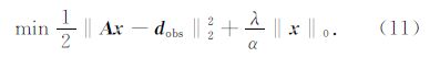
本文针对含随机噪声数据的插值问题进行研究.我们从一般的0范数正则化和优化问题出发,由迭代阈值方法推导出了加权POCS方法,证明了加权POCS方法是解无约束优化问题的一种方法,权重因子可以看作是拟合误差项的系数(Oropeza and Sacchi,2011;Gao et al.,2013).同时,我们还提出了一种改进的POCS方法来实现同时插值和去噪,该方法不需要增加任何的计算量,能够适合含噪声数据的插值.数值模拟表明,改进的POCS方法在保持POCS方法计算效率高的同时,能够很好地重建无噪声的数据和含噪声的数据.通过和先插值后去噪的结果比较,证明了同时插值和去噪的稳定性.
2 地震数据的同时插值和去噪假设地震数据的采集过程可以表示为以下的数学模型:
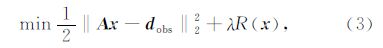
现有的基于问题(3)的大多数插值方法只是研究无噪声数据或高信噪比数据的插值,实际上问题(3)同样适合于含有随机噪声数据的插值,如果参数λ选择合适就能够实现同时插值和去噪.参数λ和迭代阈值类算法中的阈值关系紧密,直接影响阈值算法的结果.迭代阈值类算法一般都是在变换域中进行阈值运算,本质上,变换域中的阈值处理是一种去噪过程,因此基于阈值类算法的插值可以看作变换域的去噪.参数λ与噪声的能量有关,较大的噪声对应于较大的λ.如果λ选择合适,则能够达到插值效果和去噪的最佳平衡.然而不同数据的噪声能量是不同的,因此一般很难选择精确的λ.
Oropeza和Sacchi(2011)提出一种基于多道奇异谱分析的重加权替换方法,其中地震数据被重新排列为块Hankel/Toeplitz矩阵,通过降低Hankel/Toeplitz矩阵的秩来进行插值,秩的作用和λ的作用类似.该算法同样通过逐渐降低秩来实现插值,因此多道奇异谱分析方法的思想和迭代阈值法的思想是一致的.
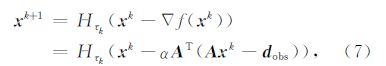
3 加权POCS方法和改进的POCS方法凸集投影法是地震插值领域最常用的方法之一,该方法计算效率高,结果稳定,非常适合大规模计算,但该方法对含噪声数据的插值效果不理想,为此Gao等(2013)提出一种加权 POCS 方法来插值含噪声数据.下面我们对加权POCS方法进行推导,证明其是解无约束优化问题的一种方法,权重因子可以看作是拟合误差项的系数.Yang等(2012)证 明了对于插值问题,迭代硬阈值法可以推导出POCS 方法.我们借鉴其中的思想推导出加权POCS方法.POCS方法可以用硬阈值迭代,也可以用软阈值迭代,取决于选用的正则算子是0范数还是1范数.本文采用硬阈值进行推导,软阈值的推导过程和硬阈值的推导过程是一样的.迭代硬阈值法的迭代公式为

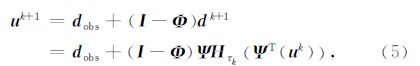
其中I 是元素全部为1的矩阵,该方法通过更新时间-空间域的解u k来得到最优解.如果POCS法的初始解为0,则POCS方法第一次迭代的解为dobs,因此POCS方法的第一次迭代就得到一个好的初始解.虽然POCS方法插值的信噪比在前几次迭代提高的很快,但是多次迭代后其最终解和迭代硬阈值法的解是一样的(Yang et al.,2012).
加权POCS方法利用加权的采样数据和加权的迭代解来构造新的迭代解(Gao et al.,2013),其中的权重因子是一个关键的参数.下面给出其推导过程,定义


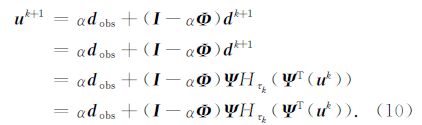
根据上述推导过程,权重因子α实际上为问题(6)中拟合误差项的系数.若问题(6)两边除以α,则问题(6)可以变为
由公式(5)可知,POCS方法得到的解 u N是d obs+(I - Φ)d N,其中 d N= Ψ(x N)是时间-空间域的迭代解.这里的(I - Φ)d N的作用是将采样点位置的元素置为0,而未被采样的点的位置的元素置为d N,则 u N的采样点位置的解为观测数据d obs,未被采样的位置的解为d N.如果观测数据d obs含有噪声,这样就会将噪声带入插值结果,因此POCS方法对于含噪声数据是不合适的.加权POCS算法的解在采样位置为α d obs+(1-α)d N,在未被采样的位置为d N,采样位置的解仍然受到含噪声的观测数据d obs的影响,此外该方法中除了需要认真选择最小阈值外,还需要权重因子α来得到好的结果.由公式(6)可知,实际上权重因子可以消去,只要选择合适的λ或最小阈值就可以实现同时插值和去噪,如果最小阈值选择合适,并且返回 d N为最终解,则可以实现同时插值和去噪,因此我们得到一种改进的POCS算法.该算法的迭代公式为

本节前两个例子用来证明改进POCS 方法对无噪声数据的插值效果;后两个例子用来证明该方法对含噪声数据插值的效果.我们用先插值后去噪的结果来验证同时插值和去噪的可靠性.本文采用 curvelet 变换为稀疏变换(Candès et al.,2006).
4.1 无噪声模拟数据的插值图 1a是一个有限差分法模拟的炮记录,时间采样个数为 256,时间采样率为 4 ms,空间采样个数为 256,道间距为 25 m.图 1b 为随机采样的数据,随机的缺失了128 道.图 2a 为POCS(uN)方法的插值结果,图 2b为图 2a与原始数据的误差.图 3a为 POCS(dN)方法的插值结果;图 3b为图 3a的残 差.这两种方法的参数一致:最小阈值为0.01,最 大迭代次数N为60.CPU时间,信噪比(SNR)和相对误差见表 1,信噪比的定义为SNR=10 log10$\frac{{||{d_{{\text{orig}}}}{\text{||}}_2^2}}{{||{d_{{\text{orig}}}}{\text{ - }}{d_{{\text{rest}}}}{\text{||}}_2^2}}$,其中d orig为原始数据,d rest为插值的数据;相对误差定义为$\frac{{||{d_{{\text{orig}}}}{\text{ - }}{d_{{\text{rest}}}}{\text{|}}{{\text{|}}_2}}}{{||{d_{{\text{orig}}}}{\text{|}}{{\text{|}}_2}}}$.这两种方法的CPU时间,信噪比和相对误差基本一致.
 |
图 1 (a)原始模拟数据;(b)随机采样的模拟数据 Fig. 1 The original synthetic data(a) and r and omly sampled synthetic data(b) |
 |
图 2 (a)POCS(u N)方法插值结果;(b)图 2a与原始数据的误差 Fig. 2 Interpolation of POCS(u N)method(a) and difference between Fig. 2a and the original data(b) |
 |
图 3 (a)POCS(d N)方法的插值结果;(b)图 3a 与原始数据的误差 Fig. 3 Interpolation of POCS(d N)method(a) and difference between Fig. 3a and the original data(b) |
| 表 1 无噪声模拟数据POCS(uN)方法和POCS(dN)方法的插值结果比较 Table 1 Interpolation of POCS(uN) and POCS(dN)for noiseless synthetic data |
图 4a为时间采样点数为600,含有115道的真 实海洋地震数据,时间采样率为 4 ms,道间距为25 m; 图 4b为图 4a随机采样的结果,共有58道被随机地去除.图 5a是原始POCS(uN)方法的插值结果;图 5b是图 5a的残差.图 6a是POCS(dN)方法的插值 结果;图 6b是图 6a的残差.同样,两种算法的参数是一致的:最小阈值为0.1,最大迭代步数N为60. 表 2给出了CPU时间,信噪比和相对误差的比较.再一次证明两种算法的计算结果和计算效率是相当的.
 |
图 4 (a)原始炮数据;(b)随机采样的炮数据 Fig. 4 The original field data(a) and r and omly sampled field data(b) |
 |
图 5 (a)POCS(uN)插值结果;(b)图 5a 与原始数据的误差 Fig. 5 Interpolation of POCS(uN)method(a) and difference between Fig. 5a and the original data(b) |
 |
图 6 (a)POCS(dN)方法的插值结果;(b)图 6a 与原始数据的误差 Fig. 6 Interpolation of POCS(dN)method(a) and difference between Fig 6a and the original data(b) |
| 表 2 无噪声真实数据POCS(uN)方法和 POCS(dN)方法插值结果比较 Table 2 Interpolation of POCS(uN) and POCS(dN)for noiseless field data |
这里POCS(uN)方法比POCS(dN)方法的结果稍微好一点,这是因为在采样位置,POCS(uN)的插 值结果被采样dobs代替了,但是这仅仅对无噪声数据是可行的.对于含噪声数据这样得到的解是不可 接受的,下面的含噪声数据插值的例子证明了这一点.
4.3 含噪声模拟数据的插值图 7a是含有零均值随机噪声的模拟数据,该数据的信噪比为4.1617 dB,图 7b是图 7a的采样结果,信噪比为1.6023 dB,采样道数为128.两种算法的最小阈值为0.17,迭代步数N为 60.图 8a是POCS(uN)的插值结果,由于仍然含有较严重噪声,因此图 8a的结果不能令人满意,图 8b是图 8a与原始数据(图 1a)的误差.图 9a给出了POCS(uN)插值结果的第3道,该道为采样道,图 9b是POCS(uN)插值的第5道,这是一个未被采样的道,可以看到采样道的插值结果不是很好.图 10a是POCS(dN)的插值结果,图 10b是图 10a与原始数据的误差.两种算法的CPU时间,信噪比和相对误差见表 3.
 |
图 7 (a)噪声模拟数据;(b)含噪声采样数据 Fig. 7 The noisy synthetic data(a) and r and omly sampled noisy synthetic data(b) |
 |
图 8 (a)POCS(uN)方法插值结果;(b)图 8a与图 1a的误差 Fig. 8 Interpolation of POCS(uN)method(a) and difference between Fig. 8a and Fig. 1a(b) |
 |
图 9 (a)POCS(uN)插值结果的第3道;(b)POCS(uN)插值结果的第5道 Fig. 9 The 3rd trace of POCS(uN)interpolation(a) and the 5th trace of POCS(uN)interpolation(b) |
 |
图 10 (a)POCS(dN)方法的插值结果;(b)图 10a与原始数据的误差 Fig. 10 Interpolation of POCS(dN)method(a) and difference between Fig. 10a and Fig. 1a(b) |
| 表 3 含噪声合成数据POCS(uN)方法和 POCS(dN)方法插值结果比较 Table 3 Interpolation of POCS(uN) and POCS(dN)for noisy synthetic data |
为了验证同时插值和去噪的可靠性,我们首先用POCS(uN)方法对图 7b进行插值,然后对插值结 果去噪.POCS(uN)方法的最小阈值为0.01,最大迭代步数N为60.插值结果见图 11a,信噪比为 5.0561 dB.对图 11a采用阈值去噪的结果见图 11b,信噪比为12.6132 dB.很明显,图 10a和图 11b的信噪比相当,因此当参数选择合适时,同时插值和去噪是稳定的.
 |
图 11 (a)POCS(uN)插值结果,最小阈值为 0.01;(b)图 11a去噪结果 Fig. 11 Interpolation of POCS(uN)with least threshold 0.01(a) and denoising result of Fig. 11a(b) |
图 12a是图 4a添加随机白噪声的结果,信噪比为5.1492 dB,图 12b是图 12a随机采样的结果,信噪比为2.34 dB.选择的最小阈值为16,最大迭代步数N为 60.图 13a是POCS(uN)的插值结果,图 13b是图 13a的残差.图 14a是 POCS(dN)的插值结果,图 14b是图 14a的残差.两种算法的CPU 时间,信噪比SNR和相对误差见表 4.由图 13a可知,POCS(uN)方法的插值结果是不可接受的,但是POCS(dN)方法可以得到较满意的结果.为了验证同时插值和去噪的可靠性,图 15a是用POCS(uN)方法的插值结果,所选的最小阈值为1,信噪比为4.9458 dB,图 15b是图 15a阈值法的去噪结果,信噪比为8.9228 dB.上述结果存在一些噪声,这是因为有效信号的部分curvelet系数和噪声的curvelet系数耦合在一起了,仅仅通过阈值类去噪算法无法消除这种现象.
 |
图 12 (a)含噪声炮数据,信噪比为5.1492 dB;(b)采样的数据,信噪比为2.34 dB Fig. 12 The noisy field data,SNR=5.1492 dB(a) and r and omly sampled noisy field data,SNR=2.34 dB(b) |
 |
图 13 (a)POCS(uN)方法插值结果;(b)图 13a 的残差 Fig. 13 Interpolation of POCS(uN)method(a) and residual of Fig. 13a (b) |
 |
图 14 (a)POCS(dN)方法的插值结果;(b) 图 14a 的残差 Fig. 14 Interpolation of POCS(dN)method(a) and residual of Fig. 14a (b) |
| 表 4 含噪声真实数据POCS(uN)方法和 POCS(dN)方法插值结果比较 Table 4 Interpolation of POCS(uN) and POCS(dN)for noisy field data |
 |
图 15 (a)POCS(uN)插值结果,最小阈值1;(b) 图 15a 的去噪结果 Fig. 15 Interpolation of POCS(uN)method with least threshold 1(a) and denoising result of Fig. 15a (b) |
根据以上的数值模拟,POCS(dN)方法的计算效率和结果得到了验证,其不仅仅适合去无噪声数据的插值,而且适合含噪声数据的插值.
5 结论本文由迭代阈值类方法推导出了加权POCS方法,证明其是解无约束优化问题的一种方法,权重因子可以看作拟合误差项的系数,同时也放大了最小阈值.本文还提出了一种改进的 POCS方法来实现同时插值和去噪,该方法只含有一个超参数(阈值),通过选择合适的阈值就能够实现插值和去噪.数值模拟表明,新的方法比原始POCS方法不增加任何计算量,在保持高效计算的同时能够很好地插值无噪声数据和含噪声数据.通过和先插值后去噪结果的比较,证明了同时插值和去噪的可靠性.
基于迭代阈值类算法进行同时插值和去噪的关键是选择合适的正则参数λ.λ和噪声的能量有直接关系,虽然可以针对每个数据的噪声能量来估计λ,但是这样做效率较低,另外本文采用最大迭代步数来控制收敛,这个迭代步数是根据我们的经验选择的,更实用的方法是选择一种自适应的停机准则来控制迭代停止.为了便于我们的推导,我们采用二维数据进行验证,本文的算法和结果对高维数据同样适用.本算法不仅仅适用于curvelet变换,其他的稀疏变换也适用于该算法框架.未来的研究方向之一是实现含噪声高维地震数据的插值和基于其他小波类变换的波场插值.关于POCS方法是解等式约束优化问题的方法的证明将在其他文章中阐述.
| [1] | Abma R, Kabir N. 2006. 3D interpolation of irregular data with a POCS algorithm. Geophysics, 71(6):E91-E97. |
| [2] | Berkhout A J, Verschuur D J. 1997. Estimation of multiple scattering by iterative inversion, Part I:Theoretical considerations. Geophysics, 62(5):1586-1595. |
| [3] | Blumensath T, Davies M E. 2008. Iterative thresholding for sparse approximations. Journal of Fourier Analysis and Applications, 14(5-6):629-654. |
| [4] | Bunks C, Saleck F M, Zaleski S, et al. 1995. Multiscale seismic waveform inversion. Geophysics, 60(5):1457-1473. |
| [5] | Candès E, Demanet L, Donoho D, et al. 2006. Fast discrete curvelet transforms. SIAM Journal on Multiscale Modeling and Simulation, 5(3):861-899. |
| [6] | Cao J J, Wang Y F, Zhao J T, et al. 2011. A review on restoration of seismic wavefields based on regularization and compressive sensing. Inverse Problems in Science and Engineering, 19(5):679-704. |
| [7] | Cao J J, Wang Y F, Yang C C. 2012. Seismic data restoration based on compressive sensing using the regularization and zero-norm sparse optimization. Chinese Journal of Geophysics(in Chinese), 55(2):596-607, doi:10.6038/j.issn.0001 5733.2012.02.22. |
| [8] | Daubechies I, Defrise M, de Mol C. 2004. An iterative thresholding algorithm for linear inverse problems with a sparsity constraint. Communications on Pure and Applied Mathematics, 57(11):1413-1457. |
| [9] | Fomel S, Liu Y. 2010. Seislet transform and seislet frame. Geophysics, 75(3):V25-V38. |
| [10] | Gao J J, Stanton A, Naghizadeh M, et al. 2013. Convergence improvement and noise attenuation considerations for beyond alias projection onto convex sets reconstruction. Geophysical Prospecting, 61(S1):138-151. |
| [11] | Geng Y, Wu R S, Gao J H. 2012. Dreamlet compression of seismic data. Chinese Journal of Geophysics(in Chinese), 55(8):2705-2715, doi:10.6038/issn.0001-5733.2012.08.023. |
| [12] | Hennenfent G, Herrmann F J. 2006. Seismic denoising with nonuniformly sampled curvelets. Computing in Science and Engineering, 8:16-25. |
| [13] | Herrmann F J, Hennenfent G. 2008. Non-parametric seismic data recovery with curvelet frames. Geophysical Journal International, 173(1):233-248. |
| [14] | Kreimer N, Sacchi M D. 2012. A tensor higher-order singular value decomposition for prestack seismic data noise reduction and interpolation. Geophysics, 77(3):V113-V122. |
| [15] | Liu B, Sacchi M D. 2004. Minimum weighted norm interpolation of seismic records. Geophysics, 69(6):1560-1568. |
| [16] | Lu J M. 1993. Principle of Seismic Exploration(in Chinese). Dongying:Petroleum University Press. |
| [17] | Ma J W. 2013. Three-dimensional irregular seismic data reconstruction via low-rank matrix completion. Geophysics, 78(5):V181-V192. |
| [18] | Mansour H, Herrmann F J, Yilmaz O. 2013. Improved wavefield reconstruction from randomized sampling via weighted one-norm minimization. Geophysics, 78(5):V193-V206. |
| [19] | Oropeza V, Sacchi M D. 2011. Simultaneous seismic data denoising and reconstruction via multichannel singular spectrum analysis. Geophysics, 76(3):V25-V32. |
| [20] | Ronen J. 1987. Wave-equation trace interpolation. Geophysics, 52(7):973-984. |
| [21] | Spitz S. 1991. Seismic trace interpolation in the f-x domain. Geophysics, 56(6):785-794. |
| [22] | Stolt R H. 2002. Seismic data mapping and reconstruction. Geophysics, 67(3):890-908. |
| [23] | Symes W W. 2007. Reverse time migration with optimal checkpointing. Geophysics, 72(5):SM213-SM221. |
| [24] | Trad D O, Ulrych T J, Sacchi M D. 2002. Accurate interpolation with high-resolution time-variant Radon transforms. Geophysics, 67(2):644-656. |
| [25] | Wang Y F. 2007. Computational Methods for Inverse Problems and Their Applications(in Chinese). Beijing:Higher Education Press. |
| [26] | Wang Y F, Cao J J, Yang C C. 2011. Recovery of seismic wavefields based on compressive sensing by an l1-norm constrained trust region method and the piecewise random subsampling. Geophysical Journal International, 187(1):199-213. |
| [27] | Xu S, Zhang Y, Lambaré G. 2010. Antileakage Fourier transform for seismic data regularization in higher dimensions. Geophysics, 75(6):WB113-WB120. |
| [28] | Yang P L, Gao J H, Chen W C. 2012. Curvelet-based POCS interpolation of nonuniformly sampled seismic records. Journal of Applied Geophysics, 79:90-99. |
| [29] | Yilmaz O. 1987. Seismic Data Processing, Investigations in Geophysics, Vol. 2. Tulsa, Okla:Society of Exploration Geophysicists. |
| [30] | Zhang H, Chen X H. 2013. Seismic data reconstruction based on jittered sampling and curvelet transform. Chinese Journal of Geophysics(in Chinese), 56(5):1637-1649, doi:10.6038/cjg20130521. |
| [31] | Zwartjes P M. 2005. Fourier reconstruction with sparse inversion. Delft:Delft University of Technology. |
| [32] | 曹静杰,王彦飞,杨长春.2012.地震数据压缩重构的正则化与零范数稀疏最优化方法.地球物理学报,55(2):596607,doi:10.6038/j.issn.00015733.2012.02.22. |
| [33] | 耿瑜,吴如山,高静怀.2012.基于Dreamlet变换的地震数据压缩理论与方法.地球物理学报,55(8):27052715,doi:10.6038/issn.00015733.2012.08.023. |
| [34] | 陆基孟.1993.地震勘探原理.东营:石油大学出版社. |
| [35] | 王彦飞.2007.反演问题的计算方法及其应用.北京:高等教育出版社. |
| [36] | 张华,陈小宏.2013.基于jitter采样和曲波变换的三维地震数据重建. 地球物理学报,56 (5):16371649,doi:10.6038/cjg20130521. |