 2015, Vol. 58


2. 桂林理工大学地球科学学院, 桂林 541004
2. College of Earth Sciences, Guilin University of Technology, Guilin 541004, China
Generally, there are three main numerical methods for the modeling of CSEM data:integral equation, finite difference, and finite element methods. Among these three methods, the finite element method with unstructured tetrahedral mesh is more suitable for simulating complex geological structures such as seafloor bathymetry. Comparing to the integral equation method, the finite element stiffness matrix is much sparser and as such the method can be used for large scale modeling of CSEM data. We adopt the node-based finite element method in this paper. For CSEM modeling, the accuracy is affected significantly by the representation of source. In order to avoid the source singularity problem caused by the total field formulation, we use the secondary field formulation and consider that the background conductivity is formed by a series of infinite horizontal layers and each with a constant conductivity value. We consider that the background conductivity is characterized by transverse anisotropy which is typically the case for marine CSEM. For the secondary field formulation, one needs to compute the background field on the mesh. We use the fast Hankel transform method to compute the background field. We adopt the classic node-based finite element method for the forward modeling. In order to avoid the spurious solution which is usually encountered in solving the Maxwell's equation directly using node-based finite element, we solve the secondary scalar and vector electromagnetic potential based on the Coulomb gauge. We re-formulated the original Maxwell's equation for the secondary scalar and vector potential. The computed background field from fast Hankel transform is converted to the primary scalar and vector potential. After applying the Galerkin finite element analysis, one can obtain a large sparse system of finite element equations. We applied the effective Dirichlet boundary condition and consider that both the scalar and vector secondary electromagnetic potential vanish on the boundary of the study domain. We solve the sparse finite element system of equations using quasi-minimum residual(QMR)method with an incomplete LU decomposition(ILU)preconditioner. Once the secondary scalar and vector potential is solved, we can compute the secondary electric and magnetic field by taking the differential of the secondary potential. The general numerical differential method can introduce significant noise. In order to solve this problem, we use a weighted moving least square method to calculate the secondary electric and magnetic field from the computed secondary potential.
To validate the effectiveness and correctness of the developed algorithm, we have implemented several model studies to compare the electromagnetic field computed from our method with the 1D analytical solution and integral equation solution. We first consider a 1D model with air and half-space as the background. We consider that there exists an infinite thin layer embedded in the half-space background. The anomalous field caused by this infinite thin layer can be computed either with finite element or fast Hankel transform. Our numerical result shows that the solution from finite element method is practically the same as the 1D analytical solution obtained from fast Hankel transform either for secondary electric or magnetic field. We have also done a comparison study for the QMR solver with Jacobian and ILU preconditioner.The result demonstrates that the convergence can be speeded up significantly by adopting the ILU preconditioner. We also consider a 3D marine reservoir model with flat bathymetry. For this model the secondary field can be effectively computed by integral equation method. As such, we have compared our results with integral equation solution for this model. In the model, we also considered the conductivity anisotropy for both reservoir and the marine sediment.Numerical result shows that the finite element solution for the problem with conductivity anisotropy is practically the same as integral equation solution. Following this, we consider a marine reservoir model with simple seafloor bathymetry represented by a trapezoidal hill. For integral equation method, we simulate this trapezoidal hill model by a staircase approximation. The numerical results show that the bathymetry effect simulated from finite element method is very close to the integral equation method especially when the receivers are far away from the bathymetry. The difference between the finite element and integral equation method can be attributed to the staircase approximation of the bathymetry for integral equation modeling. Finally, we consider a complex seafloor bathymetry model with reservoir and conductivity anisotropy. Our numerical modeling result using the finite element method have demonstrated that the observed CSEM data can be significantly distorted by the seafloor bathymetry in practical application and this effect should be addressed by robust forward modeling algorithm for the correct interpretation of subsurface geo-electric structures.
We have implemented a three-dimensional numerical modeling method for marine CSEM data using node-based finite element method based on a fully unstructured tetrahedral mesh. Comparing to the conventional structured mesh, the computation load can be significantly reduced by adopting the unstructured mesh. In the meantime, the unstructured mesh is capable of simulating complex geo-electric structures such as seafloor bathymetry. We have formulated our problem for the scalar and vector potential instead of the electric and magnetic field to address the spurious solution. In order to avoid the source singularity problem for CSEM modeling, we adopt a secondary field formulation. The sparse finite element system of equations is solved using a quasi-minimum residual method with incomplete LU decomposition result as the preconditioner to speed up the convergence. The developed algorithm was tested for several synthetic and realistic models. The numerical results have demonstrated the effectiveness of the algorithm for the modeling of complex geo-electric structures with conductivity anisotropy.
陆地可控源电磁法在油气和矿产资源勘探领域早已得到广泛应用并取得了良好的实际效果(Ward and Hohmann,1988;Zhdanov et al.,2006). 近年来,海洋电磁法(MCSEM)也被引入油气勘探领域以降低勘探风险(Srnka et al.,2006;Constable and Srnka,2007;Um and Alumbaugh,2007;Andréis and MacGregor,2008;Zhdanov,2010).在海洋环境中,受海底地形起伏和沉积因素所造成的电阻率不均匀分布和各向异性的影响,地电模型往往会非常复杂.在这种情况下,三维正演对于能否正确地解释可控源电磁数据显得至关重要( da Silva et al.,2012).目前常用的电磁三维正演方法包括有限单元法(FE)、有限差分(FD)和积分方程法(IE).积分方程法只需要对异常体区域进行剖分,因而对于简单模型中有若干局部异常体非常有效.同时,积分方程法不需要额外的边界条件.对于复杂几何形状的异常体,譬如,地形起伏、积分方程法只能用阶梯状网格来近似,且该方法所形成的矩阵为满阵,当异常体区域较大时,其模拟效率会明显降低(Zhdanov et al.,2006).有限差分法相对而言较为简单,通过有限差分法形成的总体系数矩阵为稀疏矩阵,其求解效率很高(Newman and Alumbaugh,1995),可解决积分方程中模拟大型异常区域的困难.类似于积分方程法,有限差分法也只能用规则网格对模拟区域进行剖分,对于复杂的几何形状,有限差分法只能用阶梯状网格来近似.相比基于结构化网格的有限差分和积分方程法,基于非结构化网格的有限单元法更适合于复杂电阻率模型下的可控源电磁模拟,其形成的总体系数矩阵的稀疏性和有限差分法相当,求解线性方程组的效率很高(Cai et al.,2014).有限单元法求解Maxwell方程可直接用矢量有限单元法形成关于电磁场本身的大型方程(Cai et al.,2014),也可以通过解关于位的方程来间接求取电场和磁场.相对而言,矢量有限元更为复杂,且形成的有限单元矩阵条件数更大,用迭代法求解收敛较慢(Jin,2002).
Badea等(2001)提出了一种基于Coulomb位的有限单元法井中电磁模拟算法.基于Badea所提出的方法,并考虑各向同性的全空间海水背景、各向异性的沉积岩和复杂地形因素,Puzyrev等(2013)实现了基于Coulomb电位的海洋电磁三维有限元并行模拟.取海水电导率为背景电阻率固然可简化问题,一次场也可由解析公式得到(Puzyrev et al.,2013),然而,更为真实的背景电阻率模型为层状介质.在Badea和Puzeyrev等工作的基础上,本文提出了一种以水平层状各向异性电阻率为背景的海洋电磁有限单元法三维正演,计算中采用犹他大学电磁正反演协会(CEMI)的格林库函数来计算一次场,利用COMSOL Multiphysics形成优化的非结构化四面体网格,对有限单元方程的总体系数矩阵做高效的不完全LU分解,并将结果作为QMR迭代解法的预条件因子加快收敛速度.通过对不完全LU分解预条件因子和雅克比预条件因子加以比较,我们发现QMR法的收敛效率得到了显著提高.
在文章的模型研究中,通过对比有限单元法模拟结果和解析解以及积分方程解,验证了算法的可靠性;同时,算例中也充分考虑了各向异性和地形起伏对电磁场响应的影响.
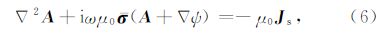
2 二次电位算法在地球物理电磁勘探领域,通常采用低频的电磁信号,忽略位移电流,采用正弦谐变时间因子e-iωt,Maxwell方程可写成如下形式:


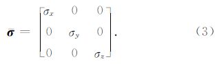
在海洋环境中由于沉积因素的影响,通常只考虑横向各向异性:σx=σy=σh为水平电导率,σz=σv为垂直电导率.
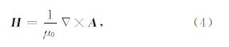
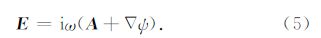
根据Coulomb位的定义,电磁场 E和H 可以写成如下形式:


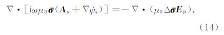
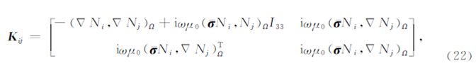
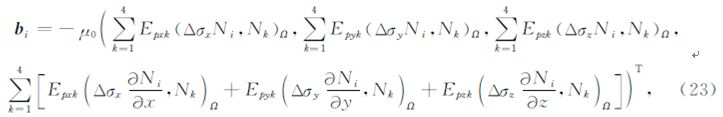
将式(13)与(14)沿x,y,z轴依次展开,利用Galerkin法将公式两端加权(Jin,2002),同时考虑矢量恒等式和散度定理,可得到如下体积分方程组:
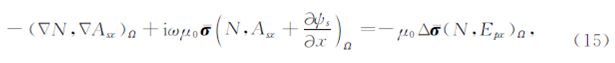


 ,N为有限单元法的形函数.用四面体单元离散整个计算区域,在各个单元中,电导率为常数,二次矢量位 As及电标量位ψs呈线性变化:


上述有限单元法求解得到的是关于电磁场的二次位(As,ψs),为了进一步得到物理意义上的电磁场(E s,H s)各分量,必须借助有效的数值微分方法来获取:

对于完全非结构化网格上的二次位,利用传统 方法得到导数的误差很大.通常采用滑动平均的方法来求取二次位的导数,设单元中位的线性描述为


为了验证文中所提方法的可靠性和有效性,这里 将以四例典型地电模型从不同角度来进行分析和阐述.
5.1 模型1:具有准解析解的一维模型背景电导率为均匀半空间模型,上半空间空气电导率为10-6S·m-1,下半空间背景电导率0.1S·m-1.从地下400 m到500 m深处为一水平方向无限延伸的高阻体,其电导率为0.01 S·m-1.沿x方向的水平电偶极源 位于(0,500,100)m处,其频率为1 Hz,偶极矩为100 Am. 一次场所对应的电导率为均匀半空间模型,相对应的二次场为水平无限延伸的高阻层所产生的,观测点位于地表y=0,z=0 处.
对于这个简单的层状模型,可以通过快速汉克 尔变换精确地得到近似于解析解的二次场(Ward and Hohmann,1988;Guptasarma and Singh,1997).在有限单元法数值模拟中,将模拟区域Ω={-4 km≤x,y<4 km,-2 km≤z≤4 km}剖分为非结构化的四面体网格(z轴向下为正).图 1为非结构化四面体网格在y=0处的断面图,网格在激发源和观测点处有所加密,网格大小可根据电磁波的趋肤深度来确定,空气中的网格较为稀疏.这个模型的单元数为 1116520,内部单元节点数为191207,方程自由度为764828,刚度矩阵维数为764828×764828.图 2为刚度矩阵稀疏特征图,不难发现虽然矩阵维数很大,但是绝大部分的元素值为0,在采取稀疏存储后刚度矩阵只需要650 M左右的存储空间.
 |
图 1 模型1的非结构化网格在y=0处的断面示意 Fig. 1 The vertical section of the unstructured mesh for Model 1 at y=0 |
 |
图 2 模型1刚度矩阵的稀疏特征 Fig. 2 The sparsity pattern of the stiffness matrix for Model 1 |
图 3和图 4分别为二次电场与磁场各个分量的有限单元数值解和通过汉克尔变换得到的准解析解的比较.其中二次电场的x,y,z分量的有限单元法解与解析解的归一化误差分别为0.6%,0.45%,0.8%.二次磁场的x,y,z分量的有限单元法解与 解析解的归一化误差分别为0.9%,0.7%,1.1%. 如前所述,在用QMR算法解有限元方程时,采用了不完全LU分解的结果作为预条件因子.图 5为采用LU预条件因子的QMR收敛曲线和采用传统雅克比预条件因子的QMR收敛曲线的比较.容易发现,采用雅克比预条件因子的QMR需要1000次迭代收敛到归一化余量为10-8,而采用不完全LU分解预条件因子的QMR仅仅需要300次迭代归一化余量就可以收敛到10-10.故而,通过改进预条件因子,迭代解法的收敛特性得到了显著提高,同时,不完全LU分解所需要的计算资源很少,甚至可以忽略不计.
 |
图 3 模型1电场的有限单元解和解析解比较. 子图a,b,c分别为二次电场的x,y,z分量 Fig. 3 A compassion of the finite element and analytical solution for the electric field for Model 1. Panel a,b and c show the x,y and z components of the secondary electric field |
 |
图 4 模型1磁场的有限单元解和解析解比较. 子图a,b,c分别为二次磁场的x,y,z分量 Fig. 4 A compassion of the finite element and analytical solution for the magnetic field for Model 1. Panel a,b and c show the x,y and z components of the secondary magnetic field |
 |
图 5 模型1的QMR迭代解收敛曲线.红色实线为采 用雅克比预条件因子的收敛曲线,蓝色星号曲线为采 用不完全LU分解的预条件因子的收敛曲线 Fig. 5 QMR convergence plot for Model 1. The solid red curve represents for QMR convergence with Jacobian preconditioner while the blue star indicates the QMR convergence with ILU preconditioner |
为简易起见和便于同积分方程结果进行比较,这里将忽略海底地形.海水深度为1 km,其各向同性电导率为3.3 S·m-1,沉积岩水平方向电导率为1 S·m-1,垂直方向电导率为0.8 S·m-1,油藏所在区域的水平方向电导率为0.01 S·m-1,垂直方向电导率为0.001 S·m-1.图 6为模型电导率在x=0和y=0处的切片图,背景电导率呈层状的空气—海水—沉积岩三层分布.有限单元法的计算模拟区域设为Ω={-5 km≤x,y<5 km,-1 km≤z≤4 km},油藏所在区域为Ωa={-1 km≤x,y<1 km,-2 km≤z≤2.1 km}.限于篇幅,略去网格剖分信息.激发源为一位于(-3000,0,900)m处,沿x方向布设的水平电偶极源,偶极矩为100 Am,激发频率为1 Hz,测线位于y=0,z=1000 m处.
 |
图 6 无地形起伏的油藏模型电导率三维切片图 Fig. 6 3D slice view of the reservoir model without seafloor bathymetry |
首先考虑各向同性模型,沉积岩和油藏区域的 电导率都为其所对应的水平方向电导率值.之后,再行考虑沉积岩和油藏电导率呈各向异性的情况.对于这样相对比较简单的油藏模型,可通过积分方程法直接计算出二次场(Zhdanov et al.,2006).图 7为模型2在电导率各向同性情况下,二次电场Ex的有限单元数值解(实部与虚部)和积分方程法解(实部与虚部)的比较.Ex分量的有限单元法解与解析解的归一化误差为0.5%.图 8为各向同性情况下,Ex的背景场和总场在y=0处的比较,油藏电导率所引起的总场畸变在图 8中清晰可见.
 |
图 7 模型2电导率各向同性情况下的FE解(红色圆 圈)和IE解(蓝色实线).子图a,b分别为电场的实部 与虚部 Fig. 7 A comparison of FE solution(red circle) and IE solution(solid blue)for Model 2 with isotropic conductivity. Panel a and b are the real and imaginary parts of the electric field |
 |
图 8 模型2在电导率各向同性情况下y=0处的背景场和总场 Fig. 8 A comparison of total and background field at y=0 for Model 2 with isotropic conductivity |
在实际的海洋环境中,由于沉积因素影响,电导 率通常情况下会呈横向各向异性,水平电导率往往大于垂向电导率.图 9为沉积层和油藏电导率均呈各向异性下的有限单元法模拟结果和积分方程模拟结果的对比,两者依然非常吻合.Ex分量的有限单元法解与解析解的归一化误差为2.3%.图 10则为背景电场Ex和总场在y=0处的比较.通过对比图 7和图 9,容易看到由电导率各向异性所引起二次场的明显畸变.因此,在实际的海洋电磁数据处理、反演以及解释中,需要考虑电导率各向异性这一重要地电特征.
 |
图 9 模型2在电导率各向异性情况下的FE解(红色圆圈)和IE解(蓝色实线).子图a,b分别为电场的实部 与虚部 Fig. 9 A comparison of FE solution(red circle) and IE solution(solid blue)for Model 2 with anisotropic conductivity. Panel a and b are the real and imaginary parts of the electric field |
 |
图 10 模型2在电导率各向异性情况下 y=0处的背景场和总场 Fig. 10 A comparison of total and background field at y=0 for Model 2 with anisotropic conductivity |
在海洋电磁勘探中,复杂的海底地形往往能引起很大的电磁场畸变.Sasaki(2011)提出了通过有限差分模拟地形和进行地形校正的算法(Sasaki,2011).为了验证算法对于地形模拟的可靠性,这里将首先考虑较为简单的梯形山模型.模型中海水深 度为1000 m,电导率为3.3 S·m-1,沉积层和油藏电 导率均为各向同性,电导率值分别为1 S·m-1和0.05 S·m-1,背景介质设为层状的空气-海水-沉积物 三层结构.为减小计算量,文中考虑较小的油藏模型位于Ωa={-500 m≤x,y<500m,2000m≤z≤2100 m},有限单元法的模拟计算区域为Ω={-5 km≤x,y<5 km,-1 km≤z≤4 km},海底地形起伏位于Ωt={-500 m≤x,y<500 m}范围内,在{-100 m≤x,y<100 m}范围内,海水深度为900 m,然后线性增加到1000 m.激发源为一位于(-1500,0,900)处、沿x方向布设的水平电偶极源,偶极矩为100 Am,激发频率为1 Hz.
图 11为梯形山示意图,其中蓝色部分代表较浅海水,红色部分代表较深海水.图 12为梯形山模型在y=0处的断面图.图 13为模型非结构化网格在y=0处的断面图,从图中可以看出网格在异常区域以及海水沉积层分界面处均做了加密.
 |
图 11 梯形山三维示意图 Fig. 11 A 3D view of the trapezoidal hill model |
 |
图 12 梯形山模型在y=0处的断面图 Fig. 12 The vertical section of the trapezoidal model at y=0 |
 |
图 13 梯形山模型非结构化网格在y=0处的断面图 Fig. 13 The vertical section of the unstructured mesh for the trapezoidal model at y=0 |
有限单元法模拟的一个很大的优点是可以用非结构化的网格精确地模拟地形.然而,积分方程只能使用结构化、相对比较规则的网格,通过积分方程法模拟地形需要用规则化的阶梯状模型来近似地形.图 14为梯形山模型的阶梯状近似,对于这种近似的地形模拟,在测点离地形相对较远时(例如航空电磁)模拟结果相对光滑可靠;测点离地形越近,由阶梯状近似所引起的离散误差越大.
 |
图 14 梯形山地形的阶梯状近似 Fig. 14 A staircase approximation for the trapezoidal hill model |
为了比较由纯地形因素引起的二次场,文中预设油藏区的电导率和沉积层电导率相同,另外,为最 大限度地减少积分方程中由阶梯状模型近似地形所带来的误差,这里将测线放在相对远离地形的水平位置z=500 m处.图 15为有限单元法和积分方程法模拟结果的比较,两种方法模拟的结果在远离地形的地方的归一化误差约为0.8%.实际的海洋电磁勘探中,接收器一般位于海底,图 16为将测点移到海底后的有限单元法和积分方程模拟结果的比较,两种方法的模拟结果的归一化误差约为15%,误差很可能是由于积分方程中用阶梯状模型近似地形所引起.
 |
图 15 无油藏的梯形山模型的有限单元解(红色圆圈)和积分方程解(蓝色实线)在水平剖面y=0,z=500 m处的比较.子图a,b分别为电场的实部与虚部 Fig. 15 A comparison of FE solution(red circle) and IE solution(solid blue)at y=0 and z=500 m for the trapezoidal hill model without reservoir. Panel a and b are the real and imaginary parts of the electric field |
 |
图 16 无油藏的梯形山模型的有限单元解(红色圆圈)和积分方程解(蓝色实线)沿地形在y=0处剖面的比较.子图a,b分别为电场的实部与虚部 Fig. 16 A comparison of FE solution(red circle) and IE solution(solid blue)at y=0 along the bathymetry for the trapezoidal hill model without reservoir. Panel a and b are the real and imaginary parts of the electric field |
接下来,文中同时考虑地形和油藏对二次场的影响,设油藏电导率为0.05 S·m-1.图 17为考虑油藏异常电导率之后有限单元法和积分方程法计算结果的比较.两种方法所得到的结果的归一化误差大约为15%.对比图 16和图 17可以得出结论,相对于油藏,地形对二次场的影响更大.
 |
图 17 含油藏的梯形山模型的有限单元解(红色圆圈)和积分方程解(蓝色实线)沿地形在y=0处剖面的 比较.子图a,b分别为电场的实部与虚部 Fig. 17 A comparison of FE solution(red circle) and IE solution(solid blue)at y=0 along the bathymetry for the trapezoidal hill model with reservoir. Panel a and b are the real and imaginary parts of the electric field |
模型4的各项参数和模型2中各向异性模型相同,相对于模型2的海水-沉积层水平分界面,模型4更为复杂.图 18为海底地形模型的三维示意图,海水深度从750 m到1000 m不等,与模型2类似,这里考虑地电背景为层状的空气-海水-沉积物三层模型,地形区域和油藏都被视为异常区.在无油藏情况下总场定义为背景场与由地形引起的二次场的总和,在有油藏和地形的情况下,总场为背景场与由地形和油藏引起的二次场总和.
 |
图 18 复杂海底地形模型三维示意图 Fig. 18 A 3D view of the model with complex seafloor bathymetry |
图 19为Ex的总场和背景场,其中黑色虚线为不含地形影响的总场.通过对比模型4的总场和不含地形的总场曲线,容易看到由地形所产生的电磁场畸变明显.将二次场振幅用一次场振幅进行归一化后可以得到图 20所示的归一化场剖面图,其中红色圆圈为带地形的二次场归一化图,黑色星号为不带地形的二次场归一化图,从中也能发现地形对电磁场的影响.
 |
图 19 模型4正演结果的总场和背景场在y=0处的比较图.蓝色实线为背景场,红色点线为含地形效应的总场,黑色虚线为不含地形效应的总场 Fig. 19 A comparison of the total field and background at y=0 for Model 4. The solid blue line represents the background field,the dotted red lines indicates the total field with seafloor bathymetry while the dashed black line is the total field without the bathymetry |
 |
图 20 模型4二次场用一次场归一化后在y=0处的比较图. 红色圆圈为带地形的归一化场,黑色星号为不 含地形的归一化场 Fig. 20 Secondary field normalized by the background field at y=0. The red circle represents the normalized field with seafloor bathymetry while the black star indicates the normalized field without the seafloor bathymetry |
本文提出了一种基于完全非结构化网格的海洋电磁有限单元三维正演算法.相比于传统的结构化网格,非结构化网格可以大大地减少计算量,同时可以模拟复杂的地电模型,譬如,海底地形.文中求解基于Coulomb规范的矢量位和标量位Maxwell方程组,利用不完全LU分解的QMR迭代算法有效提高收敛速度,采用二次场算法回避总场算法的场源奇异性,选用更符合实际情况的层状地电模型作为背景介质,讨论了地形起伏及电导率各向异性的海洋电磁三维响应规律和特征.通过对若干典型地电模型对比正演数值解与准解析解和积分方程解,验证了文中所提算法的可靠性,该算法适用于复杂三维地形和各向异性电导率介质的电磁模拟.
致谢 作者感谢美国犹他大学电磁法正反演科研组(CEMI)提供本人优良的科研环境.
| [1] | Andréis D, MacGregor L. 2008. Controlled-source electromagnetic sounding in shallow water:Principles and applications. Geophysics, 73(1):F21-F32, doi:10.1190/1.2815721. |
| [2] | Badea E A, Everett M E, Newman G A, et al. 2001. Finite-element analysis of controlled-source electromagnetic induction using Coulomb-gauged potentials. Geophysics, 66(3):786-799, doi:10.1190/1.1444968. |
| [3] | Cai H Z, Xiong B, Han M R, et al. 2014. 3D controlled-source electromagnetic modeling in anisotropic medium using edge-based finite element method. Computers & Geosciences, 73:164-176, doi:10.1016/j.cageo.2014.09.008. |
| [4] | Constable S, Srnka L J. 2007. An introduction to marine controlled-source electromagnetic methods for hydrocarbon exploration. Geophysics, 72(2):WA3-WA12, doi:10.1190/1.2432483. |
| [5] | da Silva N V, Morgan J V, MacGregor L, et al. 2012. A finite element multifrontal method for 3D CSEM modeling in the frequency domain. Geophysics, 77(2):E101-E115, doi:10.1190/geo2010-0398.1. |
| [6] | Srnka L J, Carazzone J J, Ephron M S, et al. 2006. Remote reservoir resistivity mapping. The Leading Edge, 25(8):972-975, doi:10.1190/1.2335169. |
| [7] | Freund R W, Nachtigal N M. 1991. QMR:a quasi-minimal residual method for non-Hermitian linear systems. Numer. Math., 60(1):315-339, doi:10.1007/BF01385726. |
| [8] | Guptasarma D, Singh B. 1997. New digital linear filters for Hankel J0 and J1 transforms. Geophys. Prospect., 45(5):745-762, doi:10.1046/j.1365-2478.1997.500292.x. |
| [9] | Jin J M. 2002. The Finite Element Method in Electromagnetics. 2nd ed. New Jersey:Wiley-IEEE Press. |
| [10] | Newman G A, Alumbaugh D L. 1995. Frequency-domain modelling of airborne electromagnetic responses using staggered finite differences. Geophysical Prospecting, 43(8):1021-1042, doi:10.1111/j.1365-2478.1995.tb00294.x. |
| [11] | Puzyrev V, Koldan J, de la Puente J, et al. 2013. A parallel finite-element method for three-dimensional controlled-source electromagnetic forward modelling. Geophys. J. Int., 193(2):678-693, doi:10.1093/gji/ggt027. |
| [12] | Sasaki Y. 2011. Bathymetric effects and corrections in marine CSEM data. Geophysics, 76(3):F139-146, doi:10.1190/1.3552705. |
| [13] | Um E S, Alumbaugh D L. 2007. On the physics of the marine controlled-source electromagnetic method. Geophysics, 72(2):WA13-WA26, doi:10.1190/1.2432482. |
| [14] | Um E S, Commer M, Newman G A. 2013. Efficient pre-conditioned iterative solution strategies for the electromagnetic diffusion in the Earth:finite-element frequency-domain approach. Geophys. J. Int., 193(3):1460-1473, doi:10.1093/gji/ggt071. |
| [15] | Ward S H, Hohmann G W. 1988. Electromagnetic theory for geophysical applications//Nabighian M N ed. Electromagnetic Methods in Applied Geophysics—Theory. SEG, 130-311. |
| [16] | Wu J P, Wang Z H, Li X M. 2004. Efficient Solution and Parallel Computation for Sparse Linear Systems(in Chinese). Changsha:Hunan Science and Technology Press. |
| [17] | Xu S Z. 1994. FEM in Geophysics(in Chinese). Beijing:Science Press. |
| [18] | Zhdanov M S, Lee S K, Yoshioka K. 2006. Integral equation method for 3D modeling of electromagnetic fields in complex structures with inhomogeneous background conductivity. Geophysics, 71(6):G333-G345, doi:10.1190/1.2358403. |
| [19] | Zhdanov M S. 2010. Electromagnetic geophysics:Notes from the past and the road ahead. Geophysics, 75(5):75A49-75A66, doi:10.1190/1.3483901. |
| [20] | 吴建平,王正华,李晓梅.2004.稀疏线性方程组的高效求解与并行计算.长沙:湖南科学技术出版社. |
| [21] | 徐世浙.1994.地球物理中的有限单元法.北京:科学出版社. |