 2015, Vol. 58


2. 中国海洋大学海洋地球科学学院, 青岛 266100
2. College of Marine Geosciences, Ocean University of China, Qingdao 266100, China
The curl-curl electrical field full-wave equation, which is derived from Maxwell's equations, is used as the governing equation in our marine CSEM simulation. Somerfeld radiation operator is chosen as the boundary condition on the truncated boundary. By applying the generalized variational principle to the boundary value problem of the electrical field, the equivalent variational problem is obtained. Unstructured tetrahedral grids are employed for spatial discretization in the 3D calculation domain using a non-commercial mesh generator Gmsh. Nédélec type vector basis functions are adopted for the interpolation of the electrical field within each tetrahedral element. These basis functions are divergence-free intrinsically and they guarantee the continuity of the tangential field component when crossing the interface between two different media. Unlike the nodal FE, the unknowns are assigned to the edges of the elements rather than the nodes. Substituting the electrical field by the interpolation, a system of linear equations is constructed. We solve the system of linear equations with a direct solver.
A 1D stratified air-sea-sediment model is designed for the validation of our 3D vector FE algorithm. We output the numerical solution of the electrical field of 0.01 Hz, 0.1 Hz and 1.0 Hz with three measurement configurations:inline, broadside and a 45-degree angle between the survey line and the dipole source direction. The comparison between the analytical and numerical solution shows that the relative error are less than 1% for most cases when the observation points are a few hundred meters away from the source. The CSEM response of a 2D air-sea-sediment-basement model with a horst type interface between the sediment and basement layers is then compared with the numerical solution of the well-known 2D FE algorithm MARE2DCSEM and it shows high consistency between the 2D and 3D numerical solutions. The influence of submarine topography to CSEM response is also studied. The simulation indicates that submarine topography has significant impact on the electrical field in marine CSEM. The existence of submarine topography may cover the anomalous signal induced by oil reservoir. Finally, the CSEM response to a 3D reservoir model covered by complicated submarine topography and fluctuant stratum interface is simulated and the results show that the complicated topography makes unsmooth changes to the MVO(Magnitude Versus Offset)curve.
We develop a 3D marine CSEM simulation algorithm using vector FE on unstructured meshes. The main advantages of vector FE we use in marine CSEM over regular nodal FE are:(1)no divergence correction is needed because of the vector basis functions are divergence-free;(2)the electrical field is solved directly without worrying about the discontinuity of the normal component of the electrical field. On the other hand, unstructured tetrahedral grids can easily handle complicated submarine topography and refined reservoir structures. The comparisons with 1D analytical solution and 2D numerical solution show high accuracy of our algorithm. The simulations also show that submarine topography may be an important contributor to the uncertainties of CSEM MVO anomalies.
电磁法是近地表地球物理勘探中的一种重要方法,已被广泛应用于环境监测、工程勘察、固体矿产和油气勘探等领域.进入21世纪,能源的紧缺使海洋油气勘探、开发成了各国关注的焦点.海洋地震勘探可以获得高分辨率的地下结构,指示潜在的海底油气圈闭构造,但地震剖面无法直接区分圈闭构造含油还是含水( da Silva et al.,2012).海洋可控源电磁(CSEM)勘探通过人工发射源在海底激发和测量低频电磁波可以获得海底地层的电阻率信息,从而识别高阻油气藏,降低勘探风险,提高钻井成功率.实测资料表明,有明显海洋CSEM异常的远景区,钻井成功率达70%,反之则钻井成功率将至35%以下(Hesthammer et al.,2010).近年来,ExxonMobile、Shell等国际石油公司和EMGS等海洋电磁勘探技术服务公司已在世界各海域开展了大量海洋电磁勘探工作(何展翔和余刚,2008).海洋CSEM目前的数据处理主要还是通过某一频率实测电磁场的振幅随偏移距变化曲线(MVO)和相位随偏移距变化曲线(PVO)做定性解释(Constable and Srnka,2007).要充分挖掘海洋CSEM电磁观测数据中包含的海底物性信息,对复杂海底构造的电性参数做定量分析,海洋CSEM三维反演是必不可少的,而要实现反演,首先要开发可靠的三维正演模拟算法.
现有的地球电磁三维正演模拟算法主要基于积分方程法(Hohmann,1975; Wannamaker,1991; Xiong,1992; Avdeev et al.,2002; Zhdanov et al.,2006; Avdeev and Knizhnik,2009; 殷长春和朴化荣,1994; 陈桂波等,2009; Ren et al.,2013a)、有限差分法(Newman and Alumbaugh,1995; Weiss and Constable,2006; Maa,2007; Streich,2009; 岳建华等,2008)、 有 限体积法(Haber and Ascher,2001; 杨波等,2012)、 边界单元法(Ren et al.,2013a)和有限单元法(Pridmore et al.,1981; Badea et al.,2001; da Silva et al.,2012; Puzyrev et al.,2013; Sommer et al.,2013; Weiss,2013; Koldan et al.,2014; 付长民等,2009; 徐志锋和吴小平,2010; 李勇等,2015)等方法,Avdeev(2005)和B rner(2010)对近年来地球电磁场数值模拟方法发展做了较为全面的综述,众多的数值计算方法在不同的物理问题中各有优劣,不能一概而论.本文以下主要讨论有限单元法在电磁三维数值模拟中的应用.
电磁场有限单元模拟可直接由麦克斯韦方程组求解电磁场(Schwarzbach et al.,2011; da Silva et al.,2012; Um et al.,2013; Grayver and Bürg,2014),也可以先求解库伦规范或洛伦兹规范下的电磁势,再求电磁场(Badea et al.,2001; Mukherjee and Everett,2011; Puzyrev et al.,2013; Weiss,2013; Koldan et al.,2014; 徐志锋和吴小平,2010). 求解电磁势避免了地球介质中电场的法向不连续问题,可以直接利用节点有限元方法进行求解,但由于节点有限元的插值函数不满足散度为零的条件,会产生伪解.在变分中添加罚项可以在一定程度上缓解伪解问题,但并不能完全消除,而且可能降低精度(王长清,2005),先求解电磁势再通过差分格式求解电磁场时显然也会降低数值模拟的精度(Badea et al.,2001).另一种思路是直接利用麦克斯韦方程组求解电场和磁场,若采用常规的节点有限元进行求解,会遇到三个问题:(1)电场不满足法向连续条件(徐志锋和吴小平,2010);(2)电磁场散度为零的条件得不到保证;(3)方程中旋度 算子的处理和边界条件的施加较为麻烦(Jin,2002).
为了解决以上问题,通常采用矢量有限元(或称 边有限元)方法进行求解.McMahon(1952)最早开始采用棱边单元插值形函数,但直到Nédélec(1980)发表关于矢量有限元的理论文章,并由Bossavit和Vérité(1983)成功运用于涡旋电流的计算,这种类型的插值形函数才得以受到关注并广泛应用于计算电磁学中.矢量有限元通过将待求物理量置于离散单元的边上,只要求该物理量切向连续,解决了电场法向不连续问题.同时,矢量有限元的形函数自动满足散度为零的条件,不需要在变分问题中强加散度校正项,因此矢量有限元方法在地球电磁数值模拟中备受关注.Schwarzbach等(2011)在有限元库FEMSTER的基础上发展了基于二次场的海洋可控源电磁正演.Ren等(2013b,2014b)实现了三维平面电磁波场数值模拟的自适应网格矢量有限元计算和域分解矢量有限元并行计算.Um等(2013)采用预条件迭代解法的矢量有限元方法研究了电磁场在地球介质中的扩散. Ren等(2014a)在三维平面电磁波场正演中采用了混合边界元-有限元方法,并利用快速多极子算法实现了加速.Grayver和Bürg(2014)通过将复数形式的双旋度电场方程分解为两个实型方程实现了基于六面体网格的有限元方法稳定求解.近年来国内地球电磁数值模拟中也有部分矢量有限元方面的研究.王烨(2008)研究了基于矢量有限元的高频大地电磁三维数值模拟,孙向阳等(2008)利用矢量有限元模拟了随钻测井仪在倾斜各向异性地层中的电磁响应,刘长生等(2010)实现了自适应矢量有限元的三维大地电磁正演模拟,Li等(2011)完成了中心回线激发的瞬变电磁场的矢量有限元三维正演模拟.在海洋CSEM三维数值模拟方 面,采用较多的仍是有限差分法和节点有限元方法,基于矢量有限元的三维数值模拟还未见相关文章发表.
本文从麦克斯韦方程组出发,导出关于电场的双旋度方程,利用广义变分原理求得对应的泛函,再利用矢量有限元方法在非结构四面体网格中进行求解,实现了非均匀各向同性介质中电场的求解.程序中电偶极子源的姿态可以任意设定.与一维解析解及二维有限元计算结果的对比显示了我们的算法具有较高的计算精度.同时,采用非结构四面体单元网格进行空间离散,可以模拟复杂的三维海底地形和电性结构,便于研究海底地形对实际海洋CSEM勘探的影响.
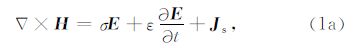
2 基本原理 2.1 边值问题时间域中的电磁场可由以下麦克斯韦方程组描述,


为了简化变分问题,通常采用理想导体(PEC)边界条件(Schwarzbach et al.,2011; Grayver et al.,2013),即n × E =0,为了达到较理想的精度,需要取非常大的计算域.这里我们采用吸收边界条件,通过构造一种m阶微分算子,将边界上电磁场的前m项抵消或湮灭,本文采用一阶算子,即索末菲辐射算子,或称为索末菲辐射边界条件(王长清,2005):

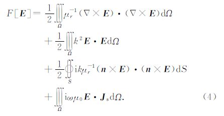
有限元方法求解边值问题的思路是将边值问题转换成对应的泛函极值问题,通过将计算域离散成有限个单元,由基函数插值得到一组有限元方程,再进行求解.由广义变分原理,可以得到与边值问题(2)—(3)对应的泛函极值问题(Jin,2002):
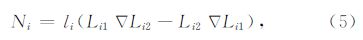
本文采用非结构四面体单元网格进行空间离散,选用Nédélec型(也称Whitney型)矢量形函数(或称基函数)(Nédélec,1980; Jin,2002):

 |
图 1 四面体单元中边的编号规则 Fig. 1 Edge definition for tetrahedral elements |
对Ni取散度,易得Δ ·Ni=0,即矢量有限元的形函数满足散度为零的条件.在每个离散的四面体单元中将插值函数(6)代入泛函(4),可得
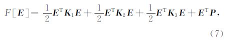
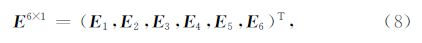
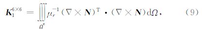
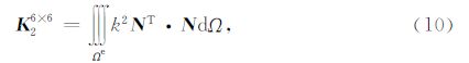
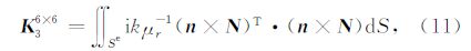
对(7)式取一阶变分即得有限元方程组
为了验证有限元算法的正确性并分析计算精度,我们设计了M1模型(空气-海水-沉积层模型),其几何与物理参数如图 2a所示.由于偶极子源产生的场具有一定的对称性,我们将有限元算法的计算域设计为圆柱体状.相比常规的六面体,在相同半径下,采用圆柱体可以减小计算域,从而减少网格节点,提高求解效率.偶极子源置于距海底50 m高 处,测线置于海底,沿x方向布置,测点间距为50 m. 图 2b是利用开源网格生成程序Gmsh(Geuzaine and Remacle,2009)生成的网格,生成网格时在源和测线附近进行了局部加密处理,最终M1模型被离散成700704个四面体,共118191个节点,821044条边.计算中采用了三种装置:(1)inline装置,即电偶极子源与测点共线,且偶极子方向与测线方向一致;(2)broadside装置,即电偶极子源与测点共线,且偶极子方向与测线方向垂直;(3)电偶极子源与测点共线,且偶极子方向与测线方向成45°夹角.我们分别计算了发射频率为0.01 Hz、0.1 Hz和1.0 Hz的偶极子源产生的电场.分配8个主频为2.4 GHz的处理器做并行计算时,单个频点的计算时间约为2.0 min.图 3给出了不同装置、不同发射频率的电场数值解与解析解的对比.
 |
图 2 (a)M1模型简图;(b)M1的离散网格 Fig. 2 (a)Sketch of the M1 model;(b)discretization of the M1 model |
 |
图 3 不同装置、不同发射频率电场数值解与解析解对比. 图中实线和虚线分别代表电场解析解的实虚部,圆圈和三角形代表电场三维数值解的实虚部,点虚线为相对误差曲线. Fig. 3 Comparisons between the numerical and analytical solutions. Solid and dashed lines represent the real and imaginary parts of the analytical electrical fields,respectively. Circles and triangles st and for the real and imaginary parts of the numerical solutions. Dash-dotted lines are the relative errors. |
在M1模型的基础上,我们设计了如图 4所示的二维模型M2.相比M1,M2多了一个电阻率为10 Ωm的基底层,基底层与沉积层之间是一个起伏界面.左侧界面距离海底1.5 km,右侧界面距离海底1.0 km,中部存在一个宽度为1.5 km的地垒状突起.这个二维模型中电偶极子源产生的电磁场无法得到精确的解析解,我们选择了将矢量有限元的数值模拟结果与国际上知名的海洋电磁二维自适应非结构有限单元程序MARE2DCSEM(Li and Key,2007)的计算结果进行对比,以验证我们程序的正确性.如图 5所示,无论是inline装置还是broadside装置,我们的计算结果都和MARE2DCSEM的吻合得很好.
 |
图 4 (a)M2模型简图;(b)MARE2DCSEM采用的二维网格,由上到下分别为空气层(红色)、 海水层(绿色)、沉积层(天蓝色)和基底(深蓝色);(c)矢量有限元正演采用的三维网格 Fig. 4 (a)Sketch of the M2 model;(b)The triangular meshes applied in 2D FE algorithm MARE2DCSEM.Layers from top to bottom are air(red),sea(green),sediment(sky blue) and basement(deep blue);(c)Tetrahedral meshes applied in our 3D simulation |
 |
图 5 三维矢量有限元与二维自适应有限元(MARE2DCSEM)计算结果对比.图中实线和虚线分别代表电场解析解的实虚部,圆圈和三角形代表电场三维数值解的实虚部 Fig. 5 Comparisons between the 3D vector FE and MARE2DCSEM solutions.Solid and dashed lines represent the real and imaginary parts of the analytical electrical fields,respectively. Circles and triangles st and for the real and imaginary parts of the numerical solutions |
实际海底地形条件远比前面讨论的模型复杂,为此有必要分析海底地形对海洋CSEM勘探实测数据的影响.为此,我们设计了如图 6所示的M3系列模型,其中M31为无油藏的水平层状模型,海水深度1000 m,M32在M31基础上加入了油藏模型,M33在M31基础上加入了一个半椭球状的凸起地形,M34则在M33的基础上添加了油藏模型.位于沉积层内的油藏利用一个高阻的扁平椭球体模拟,中心坐标为(4000,0,-2000),长半轴a=2000 m,沿x方向,b=1000 m,沿y方向,c=100 m,沿z方向.M33和M34模型中的半椭球形凸起地形位于 油藏正上方,长半轴a=2000 m,沿y方向,b=1000 m,沿x方向,c=200 m,沿z方向.电偶极子源置于(-1000,0,-950)处,根据油藏埋深,我们选择了0.75 Hz和1.0 Hz两个发射频率,分别计算了inline和broadside装置的电场.位于海底的测线沿x轴布置,范围在x=1000 m到x=7000 m之间,点距100 m.图 7所示为数值模拟结果,从图 7(a-d)M31和M32曲线可以看到,inline模式下水平层状模型中油藏引起了明显MVO异常,而broadside模式下却未能获得明显的异常,这主要是因为油藏的长半轴沿x方向,因此y方向的异常要小于x方向.M31和M33曲线的差异表明地形对电场的影响很大,M33和M34曲线的对比表明地形的存在会削弱甚至掩盖油藏产生的MVO异常,因此当采用MVO曲线对潜在油藏做定性分析时,必须考虑海底地形的影响.
 |
图 6 (a)M3系列模型简图;(b)M32模型的网格剖分,由上到下分别为空气层、 海水层和沉积层,沉积层中紫色扁椭球体为油藏模型;(c)M34模型的网格剖分 Fig. 6 (a)Sketchs of the M3 model series;(b)Meshes of the M32 model.Layers from top to bottom are air(yellow), sea(blue) and sediment(green) and reservoir(slim purple ellipsoid);(c)Meshes of the M34 model |
 |
图 7 Inline装置和broadside装置的电场MVO曲线 Fig. 7 MVO curves with inline and broadside geometries |
为了分析海底地形对海洋CSEM勘探的影响,我们设计了如图 8a所示的带海底地形的油藏模型.海水深度在931~1479 m之间,海底存在一个走向沿y轴的海岭,最大高差约为550 m,测线垂直海岭走向布置,长度为6 km(图 8b).沉积层和基底层的界面也存在地形起伏,其深度在2509~4088 m之间.位于沉积层内的油藏同样采用一个高阻的扁平椭球体模拟,其几何和物理参数与M3系列模型中的一样.为了提高数值模拟精度,在生成非结构四面体网格时对两个起伏界面的所有高程控制点均进行了加密处理,测线所在剖面也进行了网格加密,详见图 8c、8d.为了分析地形的影响和MVO曲线对海底油藏的响应,我们分别对不存在海底油藏(M41)和存在海底油藏(M42)两种情况进行了数值模拟.我们选取了0.25 Hz、0.50 Hz和0.70 Hz三个发射频率,计算结果如图 9所示.
 |
图 8 (a)带三维海底地形的海底油藏模型,图中浅蓝色平面为海平面,橙色界面为海底,紫色界面为沉积层与基地交界面;(b)海底地形及电偶极子源和测线的位置;(c)海底地形网格;(d)沉积层与基底界面地形网格 Fig. 8 (a)A reservoir model with 3D submarine and interface topographies. Interfaces from top to bottom are sea level(light blue),submarine(orange) and sediment-basement interface(purple);(b)Submarine topography and the survey geometry;(c)Meshes of the submarine topography;(d)Meshes of the interface topography between the sediment and basement |
 |
图 9 Inline和broadside装置对M41和M42模型的MVO响应曲线和测线所在剖面的地形 Fig. 9 MVO responses to Model M41 and M42 with inline and broadside geometries. Topography along the survey line is also shown in the figures |
从图 9可以发现地形起伏较大的位置,inline装置获得的电场波动也较大,这会对油藏MVO异常的提取造成干扰,而在平坦地形上MVO曲线则变得光滑.broadside装置的MVO曲线则在地形起伏区域也较为光滑,这种差异主要是由于海岭的走向造成的.Inline装置得到的是电场Ex分量,垂直于海岭走向,受地形起伏影响严重,而broadside装置得到的是平行海岭走向的Ey分量,该方向地形起伏远小于x方向,因而曲线更光滑.由趋肤深度公式($\delta \approx 503\sqrt {\rho T}$,单位m)可以得到对应于高阻油藏埋深的发射频率约为0.7 Hz,我们从图 9c上看到inline装置在发射频率0.7 Hz(对应于趋肤深度)时得到了明显的MVO异常,而0.25 Hz和0.50 Hz的MVO曲线上异常则相对较小.对于broadside装置,发射频率为0.7 Hz的MVO曲线上得到的异常也非常小,这是因为油藏的长半轴沿x方向,因此broadside装置得到的Ey对油藏的响应小于inline装置.
4 结论与讨论本文实现了基于非结构网格的海洋CSEM三维矢量有限元正演模拟.与常规的节点有限元方法相比,矢量有限元避免了电场法向不连续带来的问题,也消除了节点有限元插值基函数散度不为零带来的伪解问题,可以直接从电场的双旋度矢量方程出发求解电场.通过与一维模型的解析解及已有二维有限元计算结果对比,验证了我们的算法具有较高的计算精度.由于采用非结构四面体单元网格,我们可以模拟复杂海底地形和异常体结构的海洋CSEM响应,计算结果表明海底地形对电场影响很大,有可能掩盖深部油藏产生的MVO异常.
海洋可控源电磁数值模拟的最终目的是服务于海洋地质调查和油气勘探,而实际的海洋地质环境非常复杂,要求采用的数值计算方法在模型网格和算法实现上都要有较大的灵活性.有限差分方法的优点是简单、容易实现,但因其要求结构化的正交网格,模拟复杂地形和地质构造存在较大困难.而且正交网格不易实施局部加密处理,若对局部区域进行加密,易导致边界单元质量较差,影响计算精度.为了实现正交网格的局部加密,国际上也提出了一些 新的方法,其中一个是存在悬挂点正交网格(Bangerth et al.,2007; Bangerth and Kayser-Herold,2009),但其在算法实现上还是较为复杂.近来在地震波场数值模拟中为了应对复杂地形和地质构造发展了基于曲边网格的有限差分算法(Zhang et al.,2012; Li et al.,2015),但地球电磁场正演模拟中还未见相关研究.积分方程方法自然满足电磁场的边界条件,但实际勘探中地质异常体构造的复杂性和分布的不确定性,以及求解背景模型基本解的困难很大程度上限制了其在电磁三维数值模拟和反演中的应用.常规的节点有限元方法可以通过求解电磁势的方式实现复杂地质模型中电磁场的正演计算,但在非结构网格中,需要先利用插值方法获得差分格点的电磁势,再通过差分格式得到电磁场分量,前后两步处理都会带来计算精度的损失.采用基于非结构四面体网格的矢量有限元方法进行海洋CSEM正演模拟的一大优势是可以方便地模拟复杂的三维结构和海底地形,并直接获得电磁场.进一步提高矢量有限元计算精度需采用高阶基函数,但是Nédélec型高阶基函数不能向下兼容,即不同阶次的基函数的形式不同,因此采用高阶基函数的海洋电磁三维矢量有限元模拟还面临相当多的困难,也是下一阶段的研究方向.
致谢感谢中国海洋大学李予国教授课题组提供二维自适应非结构有限单元计算结果和两位匿名评审专家非常好的建议.
| [1] | Avdeev D B, Kuvshinov A V, Pankratov O V, et al. 2002. Three-dimensional induction logging problems, Part I:An integral equation solution and model comparisons. Geophysics, 67(2):413-426. |
| [2] | Avdeev D B. 2005. Three-dimensional electromagnetic modelling and inversion from theory to application. Surveys in Geophysics, 26(6):767-799. |
| [3] | Avdeev D, Knizhnik S. 2009. 3D integral equation modeling with a linear dependence on dimensions. Geophysics, 74(5):F89-F94. |
| [4] | Badea E A, Everett M E, Newman G A, et al. 2001. Finite-element analysis of controlled-source electromagnetic induction using Coulomb-gauged potentials. Geophysics, 66(3):786-799. |
| [5] | Bangerth W, Hartmann R, Kanschat G. 2007. Deal. II—a general-purpose object-oriented finite element library. ACM Transactions on Mathematical Software (TOMS), 33(4):Article No. 24. |
| [6] | Bangerth W, Kayser-Herold O. 2009. Data structures and requirements for hp finite element software. ACM Transactions on Mathematical Software (TOMS), 36(1):Article No. 4. |
| [7] | Börner R U. 2010. Numerical modelling in geo-electromagnetics:advances and challenges. Surveys in Geophysics, 31(2):225-245. |
| [8] | Bossavit A, Vérité J. 1983. The "TRIFOU" Code:Solving the 3-D eddy-currents problem by using H as state variable. IEEE Transactions on Magnetics, 19(6):2465-2470. |
| [9] | Chen G B, Wang H N, Yao J J, et al. 2009. Modeling of electromagnetic responses of 3-D electrical anomalous body in a layered anisotropic earth using integral equations. Chinese Journal of Geophysics (in Chinese), 52(8):2174-2181, doi:10.3969/j.issn.0001-5733.2009.08.028. |
| [10] | Constable S, Srnka L J. 2007. An introduction to marine controlled-source electromagnetic methods for hydrocarbon exploration. Geophysics, 72(2):WA3-WA12. |
| [11] | da Silva N V, Morgan J V, MacGregor L, et al. 2012. A finite element multifrontal method for 3D CSEM modeling in the frequency domain. Geophysics, 77(2):E101-E115. |
| [12] | Fu C M, Di Q Y, Wang M Y. 2009. 3D numeric simulation of marine controlled source electromagnetics (MCSEM). Oil Geophysical Prospecting (in Chinese), 44(3):358-363. |
| [13] | Geuzaine C, Remacle J F. 2009. Gmsh:A 3-D finite element mesh generator with built-in pre-and post-processing facilities. International Journal for Numerical Methods in Engineering, 79(11):1309-1331. |
| [14] | Grayver A V, Streich R, Ritter O. 2013. Three-dimensional parallel distributed inversion of CSEM data using a direct forward solver. Geophysical Journal International, 193(3):1432-1446. |
| [15] | Grayver A V, Bürg M. 2014. Robust and scalable 3-D geo-electromagnetic modelling approach using the finite element method. Geophysical Journal International, 198(1):110-125. |
| [16] | Haber E, Ascher U M. 2001. Fast finite volume simulation of 3D electromagnetic problems with highly discontinuous coefficients. SIAM Journal on Scientific Computing, 22(6):1943-1961. |
| [17] | He Z X, Yu G. 2008. Marine EM survey technology and its new advances. Progress in Exploration Geophysics (in Chinese), 31(1):2-9. |
| [18] | Hesthammer J, Stefatos A, Boulaenko M, et al. 2010. CSEM performance in light of well results. The Leading Edge, 29(1):34-41. |
| [19] | Hohmann G W. 1975. Three-dimensional induced polarization and electromagnetic modeling. Geophysics, 40(2):309-324. |
| [20] | Jin J M. 2002. The Finite Element Method in Electromagnetics. 2nd ed. New York:Wiley-IEEE Press. |
| [21] | Koldan J, Puzyrev V, de la Puente J, et al. 2014. Algebraic multigrid preconditioning within parallel finite-element solvers for 3-D electromagnetic modelling problems in geophysics. Geophysical Journal International, 197(3):1442-1458. |
| [22] | Li H, Zhang W, Zhang Z G, et al. 2015. Elastic wave finite-difference simulation using discontinuous curvilinear grid with non-uniform time step:two-dimensional case. Geophysical Journal International, 202(1):102-118. |
| [23] | Li J H, Zhu Z Q, Liu S C, et al. 2011. 3D numerical simulation for the transient electromagnetic field excited by the central loopbased on the vector finite-element method. Journal of Geophysics and Engineering, 8(4):560-567. |
| [24] | Li Y G, Key K. 2007. 2D marine controlled-source electromagnetic modeling:Part 1—An adaptive finite-element algorithm. Geophysics, 72(2):WA51-WA62. |
| [25] | Li Y, Wu X P, Lin P R. 2015. Three-dimensional controlled source electromagnetic finite element simulation using the secondary field for continuous variation of electrical conductivity within each block. Chinese Journal of Geophysics (in Chinese), 58(3):1072-1087, . |
| [26] | Liu C S, Tang J T, Ren Z Y, et al. 2010. Three-dimension magnetotellurics modeling by adaptive edge finite-element using unstructured meshes. Journal of Central South University (Science and Technology) (in Chinese), 41(5):1855-1859. |
| [27] | Maa F A. 2007. Fast finite-difference time-domain modeling for marine-subsurface electromagnetic problems. Geophysics, 72(2):A19-A23. |
| [28] | McMahon J. 1952. Lower bounds for the electrostatic capacity of a cube. Proceedings of the Royal Irish Academy. Section A:Mathematical and Physical Sciences, 55:133-167. |
| [29] | Mukherjee S, Everett M E. 2011. 3D controlled-source electromagnetic edge-based finite element modeling of conductive and permeable heterogeneities. Geophysics, 76(4):F215-F226. |
| [30] | Nédélec J C. 1980. Mixed finite elements in [WTHT]R[WTBZ]3. Numerische Mathematik, 35(3):315-341. |
| [31] | Newman G A, Alumbaugh D L. 1995. Frequency-domain modelling of airborne electromagnetic responses using staggered finite differences. Geophysical Prospecting, 43(8):1021-1042. |
| [32] | Pridmore D F, Hohmann G W, Ward S H, et al. 1981. An investigation of finite-element modeling for electrical and electromagnetic data in three dimensions. Geophysics, 46(7):1009-1024. |
| [33] | Puzyrev V, Koldan J, de la Puente J, et al. 2013. A parallel finite-element method for three-dimensional controlled-source electromagnetic forward modelling. Geophysical Journal International, 193(2):678-693. |
| [34] | Ren Z Y, Kalscheuer T, Greenhalgh S, et al. 2013a. Boundary element solutions for broad-band 3-D geo-electromagnetic problems accelerated by an adaptive multilevel fast multipole method. Geophysical Journal International, 192(2):473-499. |
| [35] | Ren Z Y, Kalscheuer T, Greenhalgh S, et al. 2013b. A goal-oriented adaptive finite-element approach for plane wave 3-D electromagnetic modelling. Geophysical Journal International, 194(2):700-718. |
| [36] | Ren Z Y, Kalscheuer T, Greenhalgh S, et al. 2014a. A hybrid boundary element-finite element approach to modeling plane wave 3D electromagnetic induction responses in the Earth. Journal of Computational Physics, 258:705-717. |
| [37] | Ren Z Y, Kalscheuer T, Greenhalgh S, et al. 2014b. A finite-element-based domain-decomposition approach for plane wave 3D electromagnetic modeling. Geophysics, 79(6):E255-E268. |
| [38] | Schenk O, Gärtner K. 2004. Solving unsymmetric sparse systems of linear equations with PARDISO. Future Generation Computer Systems, 20(3):475-487. |
| [39] | Schwarzbach C, Börner R U, Spitzer K. 2011. Three-dimensional adaptive higher order finite element simulation for geo-electromagnetics—a marine CSEM example. Geophysical Journal International, 187(1):63-74. |
| [40] | Sommer M, Hölz S, Moorkamp M, et al. 2013. GPU parallelization of a three dimensional marine CSEM code. Computers & Geosciences, 58:91-99. |
| [41] | Streich R. 2009. 3D finite-difference frequency-domain modeling of controlled-source electromagnetic data:Direct solution and optimization for high accuracy. Geophysics, 74(5):F95-F105. |
| [42] | Sun X Y, Nie Z P, Zhao Y W, et al. 2008. The electromagnetic modeling of logging-while-drilling tool in tilted anisotropic formations using vector finite element method. Chinese Journal of Geophysics (in Chinese), 51(5):1600-1607, doi:10.3321/j.issn:0001-5733.2008.05.036. |
| [43] | Um E S, Commer M, Newman G A. 2013. Efficient pre-conditioned iterative solution strategies for the electromagnetic diffusion in the Earth:finite-element frequency-domain approach. Geophysical Journal International, 193(3):1460-1473. |
| [44] | Wang C Q. 2005. Advanced Computational Electromagnetics (in Chinese). Beijing:Peking University Press. |
| [45] | Wang Y. 2008. A study of 3D high frequency magnetotellurics modeling by edge-based finite element method [Ph. D. thesis] (in Chinese). Changsha:Central South University. |
| [46] | Wannamaker P E. 1991. Advances in three-dimensional magnetotelluric modeling using integral equations. Geophysics, 56(11):1716-1728. |
| [47] | [JP3]Weiss C J, Constable S. 2006. Mapping thin resistors and hydrocarbons with marine EM methods, Part II—Modeling and analysis in 3D. Geophysics, 71(6):G321-G332. |
| [48] | [JP3]Weiss C J. 2013. Project APhiD:A Lorenz-gauged A-Φ decomposition for parallelized computation of ultra-broadband electromagnetic induction in a fully heterogeneous Earth. Computers & Geosciences, 58:40-52. |
| [49] | Xiong Z H. 1992. Electromagnetic modeling of 3-D structures by themethod of system iteration using integral equations. Geophysics, 57(12):1556-1561. |
| [50] | Xu Z F, Wu X P. 2010. Controlled source electromagnetic 3-D modeling in frequency domain by finite element method. Chinese J. Geophys. (in Chinese), 53(8):1931-1939, doi:10.3969/j.issn.0001-5733.2010.08.019. |
| [51] | Yang B, Xu Y X, He Z X, et al. 2012. 3D frequency-domain modeling of marine controlled source electromagnetic responses with topography using finite volume method. Chinese Journal of Geophysics (in Chinese), 55(4):1390-1399, doi:10.6038/j.issn.0001-5733.2012.04.035. |
| [52] | Yin C C, Piao H R. 1994. Three-dimensional electromagneticmodelling and its application in frequency-domain electromagnetic sounding methods. Acta Geophysica Sinica (in Chinese), 37(6):820-827. |
| [53] | Yue J H, Yang H Y, Hu B. 2008. 3D finite difference time domain numerical simulation for TEM in-mine. Progress in Geophysics [LL] (in Chinese), 22(6):1904-1909, doi:10.3969/j.issn.1004-2903.2007.06.036. |
| [54] | Zhang W, Zhang Z G, Chen X F. 2012. Three-dimensional elastic wave numerical modelling in the presence of surface topography by a collocated-grid finite-difference method on curvilinear grids. Geophysical Journal International, 190(1):358-378. |
| [55] | Zhdanov M S, Lee S K, Yoshioka K. 2006. Integral equation method for 3D modeling of electromagnetic fields in complexstructures with inhomogeneous background conductivity. Geophysics, 71(6):G333-G345 |
| [56] | 陈桂波,汪宏年,姚敬金等.2009.用积分方程法模拟各向异性地层中三维电性异常体的电磁响应.地球物理学报,52(8):2174-2181,doi:10.3969/j.issn.00015733.2009.08.028. |
| [57] | 付长民,底青云,王妙月.2009.海洋可控源电磁法三维数值模拟.石油地球物理勘探,44(3):358-363. |
| [58] | 何展翔,余刚.2008.海洋电磁勘探技术及新进展.勘探地球物理进展,31(1):2-9. |
| [59] | 李勇,吴小平,林品荣.2015.基于二次场电导率分块连续变化的三维可控源电磁有限元数值模拟.地球物理学报,58(3):1072-1087,doi:10.6038/cjg20150331. |
| [60] | 刘长生,汤井田,任政勇等.2010.基于非结构化网格的三维大地电磁自适应矢量有限元模拟.中南大学学报(自然科学版),41(5):1855-1859. |
| [61] | 孙向阳,聂在平,赵延文等.2008.用矢量有限元方法模拟随钻测井仪在倾斜各向异性地层中的电磁响应.地球物理学报,51(5):1600-1607,doi:10.3321/j.issn:0001-5733.2008.05.036. |
| [62] | 王长清.2005.现代计算电磁学基础.北京:北京大学出版社. |
| [63] | 王烨.2008.基于矢量有限元的高频大地电磁法三维数值模拟[博士论文].长沙:中南大学. |
| [64] | 徐志锋,吴小平.2010.可控源电磁三维频率域有限元模拟.地球物理学报,53(8):1931-1939,doi:10.3969/j.issn.0001-5733.2010.08.019. |
| [65] | 杨波,徐义贤,何展翔等.2012.考虑海底地形的三维频率域可控源电磁响应有限体积法模拟.地球物理学报,55(4):1390-1399,doi:10.6038/j.issn.0001-5733.2012.04.035. |
| [66] | 殷长春,朴化荣.1994.三维电磁模拟技术及其在频率测探法中应用.地球物理学报,37(6):820-827. |
| [67] | 岳建华,杨海燕,胡搏.2008.矿井瞬变电磁法三维时域有限差分数值模拟.地球物理学进展,22(6):1904-1909,doi:10.3969/j.issn.1004-2903.2007.06.036. |