 2015, Vol. 58


This paper analyzes the advantages of magnetic field intensity in multi-source ground-airborne transient electromagnetic interpretation and puts forward multi-source and multi-component full field apparent resistivity algorithm for each component on the basis of inverse function theorem and iterative method. The results of theoretical models show that the first and last part of the apparent resistivity curve can reach the resistivity of the first and the last layer, respectively. Thus, multi-component, full time and full space apparent resistivity definition is achieved.The results of layered models show that:(1)Full field apparent resistivity can tell the underground electric change smoothly, completely and gradually.(2)When the resistivity of layered model changes, the differentiation of full field apparent resistivity is obvious, which can easily and intuitively identify electric layer.(3)With the change of offset, the difference among apparent resistivity curves of each component is small and they all reflect subsurface structure well.(4)As receiver altitude, offset and time are considered simultaneously in our calculation, full field apparent resistivity can achieve full space and full time apparent resistivity calculation. The results of three dimensional model with a low-resistivity anomaly show that:(1)By changing spatial location and current direction of the galvanic sources, signal intensity of different components can be strengthened or weakened.(2)Full field apparent resistivity sections of each component can all match well with the designed complex model.
This paper focuses on multi-component full field apparent resistivity calculation of multi-source ground-airborne transient electromagnetic method with galvanic sources. Full field apparent resistivity algorithm, which is based on inverse function theorem and iterative method, realizes multi-component, full time and full space apparent resistivity calculation and can completely, smoothly and gradually tell the subsurface electrical variations. By changing the spatial location and current direction of galvanic sources, the results of three dimensional model confirm that multi-source ground-airborne transient electromagnetic method with galvanic sources surely can strengthen signal intensity and improve signal-to-noise ratio. Besides, the effectiveness of multi-component full field apparent resistivity algorithm with magnetic field intensity for multi-source ground-airborne transient electromagnetic method with galvanic sources is also verified.
地空瞬变电磁法已成功应用在地热调查、火山结构、地下水盐渍化及地下水监测等领域(Mogi et al.,1998,2009;Allah et al.,2011;Ito et al.,2013;李肃义等,2013;嵇艳鞠等,2013;Wang等,2013),由于电性源地空系统仍属时间域电磁法的范畴,且时间域电磁法特别适合深部、隐伏矿床勘查(周平和施俊法,2007;陈贵生,2006),因此该法在矿产勘探中也具备较大的发展潜力.目前我国的矿业形势十分严峻,一方面老矿山的储量日趋枯竭,另一方面新发现的矿床又越来越少,因此国家明确提出了危机矿山和第二深度空间探矿的专项计划,这两项专项计划针对的都是大深度问题,都要求矿产勘查向深部发展(滕吉文,2010;王金亮等,2010).根据Mogi等(2009),目前已知的电性源地空系统的最大探测深度可达800 m,若采用多辐射场源,还可进一步提高该法的探测深度,将瞬变电磁法引入到深部探测.另一方面矿产勘查工作迫切需要向地形复杂的山区等尚未被详细探查的区域发展,由于地空瞬变电磁法在空中进行数据采集,可实现阵列式观测及三维信息采集,相比较地面瞬变电磁法在这些地区具有更大的可操作性.
到目前为止,电性源地空系统仍采用单辐射源工作模式,数据解释工作大都仍基于地面LOTEM(李肃义等,2013;嵇艳鞠等,2013),李貅等(2015)结合TEM三维拟地震解释技术,建立了地空逆合成孔径成像的三维解释理论体系.关于电性源地空系统的研究工作多集中在数据校正以及设备研发方面,校正工作包括有运动校正、消除当地噪声,基线漂移校正、去噪等(Mogi等,1998,2009;李肃义等,2013),Verma等(2010)分析了飞行高度、偏移距等参数对电性源地空系统响应特征的影响.目前得到成功应用的系统有两套,一套是Mogi主持研发的直升机平台的GREATEM系统,它采用磁力计直接测量磁感应强度B(t),该系统已成功应用于地热调查及火山结构调查(Mogi等,1998,2009;Allah等,2011;Ito等,2013);另一套是吉林大学自主研制的飞艇搭载的电性源发射系统,该系统采集的是电压响应,它与磁感应强度对时间的变化率∂B(t)/∂t成正比,该系统在地下水盐渍化及地下水监测方面取得了良好的应用效果(李肃义等,2013;嵇艳鞠等,2013;Wang et al.,2013).目前对多辐射源地空瞬变电磁法的研究工作尚未展开,解决了全时域、全空域的多分量全域视电阻率定义问题,不仅可以提供一种定性的、直观的初步解释方法,为三维解释技术以及反演提供更丰富的信息,还可利用各分量各自的特点更好地反映地下电性信息.
当遇到良导目标体时,与B(t)相比,∂B(t)/∂t会很快衰减到噪声水平之下(Grant,1965),这会限制电性源地空系统的探测深度;而B(t)作为∂B(t)/∂t关于t的积分,虽然对于浅部的分辨能力要相对弱一些,但是由于B(t)衰减慢,在晚期时幅值仍较大,因此在晚期仍有较高的分辨率(Smith and Annan,1998).另一方面,通过计算分析我们发现,以B(t)定义的电阻率参数的函数形态要相对简单,而∂B(t)/∂t不仅是多解函数,它还会带来诸如“overshoot”和“undershoot”的假异常干扰(Spies and Eggers,1986),相对于∂B(t)/∂t,利用B(t)进行多辐射源地空系统数据解释具有其独特的优势.目前,由于受到制作工艺和使用范围等方面的限制,在地空系统设备中使用磁力计仍需解决航空电磁法中存在的诸如高温、带宽等问题(Foley and Leslie,1998),可以采用对∂B(t)/∂t进行积分求取B(t)的方法进行数据解释(许建荣等,2008).鉴于多辐射场源本身存在的诸多优势,如通过调整源的位置及电流方向,可加强采集信号强度、削弱随机噪声、减少电性源体积效应的影响、更全面反映地下异常体位置信息等,若再结合B(t)进行多分量数据解释,应会进一步提高地空系统的探测深度以及分辨率.
2 理论与分析2.1 多辐射场源地空系统理论图 1a所示为均匀大地地表电偶极子所在坐标系示意图,AB表示位于地表的电偶极子,电偶极子的中心即为坐标系原点o,z轴指向大地,整个坐标系满足右手坐标系准则,M表示空中任意位置的测点,它与o之间距离为R,M在地表的投影为P,P与o之间距离为r,即本文中提及的偏移距.图 1b所示为多辐射场源的坐标系俯视图,AiBi表示第i个电性源,电流方向见图中箭头所示,由于实际应用中铺设的电性源可能长达数公里,因此我们采用了对电性源进行剖分,采用有限求和的方法进行计算,相应的多辐射场源均匀大地地表电性源在空中产生的频率域总磁感应强度Bp(ω)(p=x,y,z)如(1)式所示(朴化荣,1990).

|
图 1 坐标系示意图 (a)地表电性源坐标系示意图;(b)多辐射源剖分俯视图. Fig. 1 Sketch of coordinate system (a)Sketch of wire source on the ground;(b)Top view of multi-source subdivision. |
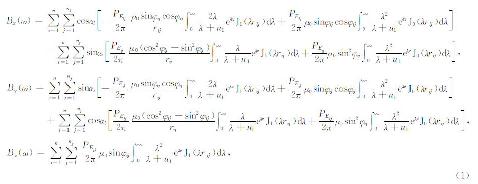
 ,k12=-iωμσ1-ω2με,k1是介质的波数,αi表示第i个电性源与第1个电性源之间的矢量夹角,φij和rij分别表示对应第i个电性源剖分的第j个电偶极子对应的夹角和偏移距,n表示电性源的总个数,ni表示第i个电性源的剖分个数,J0和J1分别表示零阶、一阶贝塞尔函数.
当使用阶跃波作为发射波形时,时间域的场可以由频率域的场通过正、余弦变换得到,见(2)式(Kaufman and Keller,1987;李貅,2002).

进行视电阻率定义,首先要知道场与电阻率之间的函数关系,为了使分析不失一般性,我们采用了两个相交的源对多辐射场源地空系统场的特征进行分析,源以及测点坐标的俯视图见图 2.

|
图 2 均匀半空间模型双源地空系统坐标系俯视图 Fig. 2 Top view of double sources and survey points |
计算采用的参数如下:源1和源2的长度均为1000 m,电流方向如图中箭头所示,两个源之间的夹角为30°,电流大小均为500 A;观察点M1和M2处于飞行高度100 m处,距离源1的偏移距分别为500和5000 m,在x1 y1 z1坐标系中对应的坐标分别为(300 m,400 m,-100 m)和(3000 m,4000 m,-100 m).图 3和4所示分别为均匀半空间模型下,多辐射源地空系统在不同偏移距下,电磁响应和磁感应强度随电阻率的变化曲线.从图 3中可以看出,在电阻率(0.001~10000 Ωm)变化范围内,无论是小偏移距(500 m)还是大偏移距(5000 m)情况下,∂Bp(t)/∂t(p=x,y,z)随电阻率变化的曲线形态复杂,且x、y、z三个分量基本上都是关于电阻率参数的多值函数;从图 4中可以看出,Bz(t)在小、大偏移距情况下,在任何时刻均可视为半空间电阻率参数的单调函数,而Bp(t)(p=x,y)的情况与 ∂Bp(t)/∂t(p=x,y,z)类似,Spies和Eggers(1986)已经证实,使用∂B(t)/∂t做视电阻率定义会带来类似于“overshoot”和“undershoot”的假异常,而使用B(t)得到的视电阻率曲线能够平滑、渐变地反映出地下的电性信息(Yang,1986).因此对于多辐射场源地空系统瞬变电磁法,使用B(t)做视电阻率定义具有更大的优势.

|
图 3 不同偏移距下磁场响应∂Bp(t)/∂t(p=x,y,z)在不同时刻随均匀半空间模型电阻率变化 (a)偏移距500 m,∂Bx(t)/∂t;(b)偏移距500 m,∂By(t)/∂t;(c)偏移距500 m,∂Bz(t)/∂t;(d)偏移距5000 m,∂Bx(t)/∂t;(e)偏移距5000m,∂By(t)/∂t;(f)偏移距5000 m,∂Bz(t)/∂t. Fig. 3 ∂Bp(t)/∂t(p=x,y,z) at different time gates with variation of half space resistivity with short and long offset (a)Offset 500 m,∂Bx(t)/∂t;(b)Offset 500 m,∂By(t)/∂t;(c)Offset 500 m,∂Bz(t)/∂t; (d)Offset 5000 m,∂Bx(t)/∂t;(e)Offset 5000 m,∂By(t)/∂t;(f)Offset 5000 m,∂Bz(t)/∂t. |

|
图 4 不同偏移距下磁场响应Bp(t)(p=x,y,z)在不同时刻随均匀半空间模型电阻率变化 (a)偏移距500 m,Bx(t);(b)偏移距500 m,By(t);(c)偏移距500 m,Bz(t); (d)偏移距5000 m,Bx(t);(e)偏移距5000 m,By(t);(f)偏移距5000 m,Bz(t). Fig. 4 Bp(t)(p=x,y,z) at different time gates with variation of half space resistivity with short and long offset (a)Offset 500 m,Bx(t);(b)Offset 500 m,By(t);(c)Offset 500 m,Bz(t); (d)Offset 5000 m,Bx(t);(e)Offset 5000 m,By(t);(f)Offset 5000 m,Bz(t). |
由于多辐射场源地空系统磁感应强度与电阻率参数之间存在复杂的隐函数关系,导致无法直接得到一个用磁感应强度表示的显式关系式来表达视电阻率.但考虑到Bz(t)是关于电阻率的单调减函数,而Bp(t)(p=x,y)和∂Bp(t)/∂t(p=x,y,z)是关于电阻率的双值函数,该双值函数可以看成是两个单调函数的组合,这就为基于反函数定理思想定义视电阻率创造了条件,本文基于反函数定理提出全域视电阻率定义方法,在视电阻率计算过程中同时考虑到位置坐标、时间等各个参数,实现时间上不分早晚、距离上不分远近的视电阻率定义.
3.1 用磁感应强度的z分量定义视电阻率由于Bz(t)是关于电阻率的单调函数,根据反函数定理知,必然存在一个电阻率值唯一地对应着一个Bz(t)值,为此,可以采用泰勒展开的办法,将磁感应强度的积分表达式展成级数形式,取其线性主部,建立起迭代关系的视电阻率定义式.
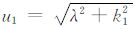
将磁感应强度的z分量记为Bz(ρ,C,t),其中C表示空中测点的位置坐标参数.为保证较快收敛,建议按照实际应用情况,用电阻率覆盖范围内的一个中间值作为初值ρτ(0).在ρτ(0)的邻域内对Bz(ρ,C,t)进行泰勒展开

在该邻域内保留(3)式的前两项,有
对(4)式进行变换


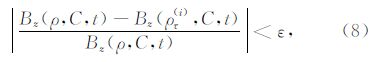
(7)式的迭代终止条件为

|
图 5 磁感应强度z分量全域视电阻率定义方法流程图 Fig. 5 Flow chart of full field apparent resistivity definition for Bz(t) |
大量模型计算表明,Bp(t)(p=x,y)是关于电阻率的双解问题,首先需要找到极值点所在位置,然后再在极值点两侧分别求取这两个解.进一步的研究表明,如果想从Bp(t)(p=x,y)数据中得到光滑渐变完整的视电阻率曲线,还需要将双解问题进一步分解为以下三种情况:当两个解相差较小时(如10%),对这两个解取平均作为该时间道的解;当两个解相差较大时(如300%),选择与相邻时间道的解更接近的解作为该时间道的解;其他情况均视为无合适解问题.对于无合适解问题,为了得到完整的视电阻率曲线,本文采用最小曲率插值方法对空缺的数据进行补足,该法能够保证曲线按最小曲率变化且保持曲线光滑,无约束点原位最小曲率差分迭代算法见(9)式(王万银等,2009).
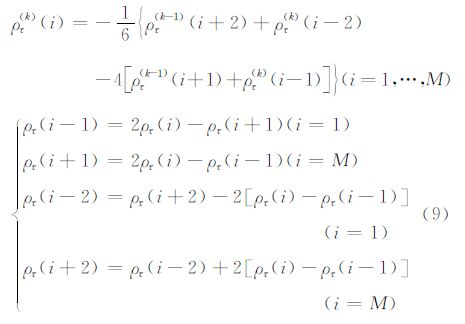
其中k表示迭代的次数,M表示参与插值的总个数,一般在需要插值的区域左右两端各取2个点参与计算.利用Bp(t)(p=x,y)进行视电阻率定义的流程图见图 6.

|
图 6 磁感应强度x和y分量全域视电阻率定义方法流程图 Fig. 6 Flow chart of full field apparent resistivity definition for Bp(t)(p=x,y) |
图 7所示为由By(t)求得的视电阻率曲线进行补足前后的对比图,模型参数如下:电阻率分别为ρ1=100 Ωm,ρ2=10 Ωm,ρ3=100 Ωm,层厚h1=20 m,h2=10 m,源1、2的长度均为1000 m,电流方向如图中箭头所示,两源之间的夹角为30°,电流大小均为500 A,观察点位于空中100 m处,距源1的偏移距为500 m,在x1y1z1坐标系中对应的坐标为(300 m,400 m,-100 m).图 7b中空白的那段曲线对应无合适解问题,与图 7c对比可以看出,经过最小曲率补足后,得到的视电阻率曲线能够光滑渐变完整地反映出所设计模型的电性变化,而且由于该法可以保证曲线按照最小曲率光滑变化,该法适合对B(t)定义的视电阻率曲线进行补足.

|
图 7 进行最小曲率补足前后的全域视电阻率对比图(模型和计算参数:源1、2的长度均为1000 m,两源夹角30°,电流大小均为500 A,观测点位于飞行高度100 m处,距源1的偏移距为500 m,在x1 y1 z1坐标系中对应的坐标为(300 m,400 m,-100 m))(a)电性源及测点坐标俯视图;(b)补足前;(c)补足后. Fig. 7 Comparison of full field apparent resistivity before and after minimum curvature interpolation(Parameters: The lengths of source 1 and 2 are both 1000 m,with an angle of 30° and transmitting current 500 A. Coordinates of survey point with an offset of 500 m in x1 y1 z1 coordinate system are(300 m,400 m,-100 m))(a)Top view of sources and survey point;(b)Before interpolation;(c)After interpolation. |
设计了改变第二层电阻率的二层模型对第3节中提及的多分量全域视电阻率定义方法进行验证,模型参数如下:源1、2的长度均为1000 m,电流方向如图中箭头所示,两源之间的夹角为30°,电流大小均为500 A,观测点位于飞行高度100 m处,距源1的偏移距为500 m,在x1 y1 z1坐标系中对应的坐标为(300 m,400 m,-100 m),二层模型第一层的电阻率ρ1=100 Ωm,层厚h1=20 m,改变第二层的电阻率ρ2=2,5,10,30,80,200,500,800 Ωm.使用Bp(t)(p=x,y,z)定义的多分量全域视电阻率曲线见图 8,可见随着第二层电阻率的变化,视电阻率曲线呈现出有规律的变化,不仅能够在早期和晚期逐渐趋于模型的第一层和最后一层电阻率,还能够完整渐变光滑地反映出模型的电性信息变化.

|
图 8 偏移距500 m时用Bp(t)(p=x,y,z)定义的全域视电阻率曲线(模型和计算参数:源1、2的长度均为1000 m,两源夹角30°,电流大小均为500 A,观测点位于飞行高度100 m处,距源1的偏移距为500 m,在x1 y1 z1坐标系中对应的坐标为(300 m,400 m,-100 m))(a)电性源及测点坐标俯视图;(b)Bx(t)所得的视电阻率曲线;(c)By(t)所得的视电阻率曲线;(d)Bz(t)所得的视电阻率曲线. Fig. 8 Full field apparent resistivity from Bp(t)(p=x,y,z) with an offset of 500 m(Parameters: The lengths of source 1 and 2 are both 1000 m,with an angle of 30° and transmitting current 500 A. Coordinates of survey point with an offset of 500 m in x1 y1 z1 coordinate system are(300 m,400 m,-100 m))(a)Top view of sources and survey point;(b)Apparent resistivity from Bx(t);(c)Apparent resistivity from By(t); (d)Apparent resistivity from Bz(t). |
为了说明偏移距对多辐射源地空系统全域视电阻率的影响,设计了如下模型:源1、2的长度均为1000 m,电流方向如图中箭头所示,两源之间的夹角为30°,电流大小均为500 A,观测点位于飞行高 度100 m处,距离源1的偏移距分别为500 m、1500 m、3000 m和5000 m,在x1 y1 z1坐标系中对应的坐标分别为(300 m,400 m,-100 m),(1060 m,1060 m,-100 m),(2121 m,2121 m,-100 m)和(3000 m,4000 m,-100 m),三层模型的电阻率ρ1=500 Ωm,ρ2=100 Ωm,ρ3=500 Ωm,层厚h1=800 m,h2=800 m. 从图 9中可以看出,全域视电阻率定义方法同时适用于大偏移距和小偏移距,曲线均能完整渐变光滑地反映出地下的电性信息变化,在早期和晚期分别趋近于模型的首层和底层电阻率,解决了多辐射场源地空系统视电阻率定义距离上不分远近的问题,且通过比较可以看出偏移距变化对各分量视电阻率曲线的分异均较小.

|
图 9 偏移距变化对多辐射场源地空系统多分量全域视电阻率曲线的影响(模型和计算参数:源1、2的长度均为1000 m,两源夹角30°,电流大小均为500 A,观测点位于飞行高度100 m处,距离源1的偏移距分别为500 m、1500 m、3000 m、 5 000 m) (a)电性源及测点坐标俯视图;(b)偏移距对Bx(t)视电阻率曲线的影响;(c)偏移距对By(t)视电阻率曲线的影响; (d)偏移距对Bz(t)视电阻率曲线的影响. Fig. 9 Influence of offset on multi-component apparent resistivity definition of multi-source ground-airborne transient electromagnetics(Parameters: The lengths of source 1 and 2 are both 1000 m,with an angle of 30° and transmitting current 500 A. Offsets of the survey points are 500 m,1500 m,3000 m and 5000 m,respectively) (a)Top view of sources and survey points;(b)Influence of offset on apparent resistivity from Bx(t);(c)Influence of offset on apparent resistivity from By(t);(d)Influence of offset on apparent resistivity from Bz(t). |
为了验证多辐射场源地空系统相对于单辐射源地空系统的优势,设计了如下三维模型:在电阻率为100 Ωm的均匀大地中,赋存一个埋深为90 m,电阻率为10 Ωm、尺寸为100 m×100 m×20 m的板状体,见图 10,计算采用的源的长度均为110 m,电流大小50 A,接收高度-80 m,三维正演采用矢量有限元方法完成.

|
图 10 模型示意图 (a)低阻体模型示意图;(b)低阻体尺寸参数示意图. Fig. 10 Model sketch (a)Anomalous body sketch;(b)Size of anomalous body. |
图 11(a—d)所示为单辐射场源情况下模型俯视图以及Line32(y=0 m)测线的各分量多测道图,从图中可以看出,x分量多测道图会出现变号,y和z分量多测道图形态类似,由一系列单峰曲线构成,幅值上以z分量为最大.

|
图 11 单辐射场源情况下Line32(y=0 m)各分量多测道图 (a)单辐射场源俯视图;(b)单辐射场源x分量衰减电压多测道图;(c)单辐射场源y分量衰减电压多测道图;(d)单辐射场源z分量衰减电压多测道图. Fig. 11 Multi-component multi-channel figure of Line32(y=0 m)with single source model (a)Top view of single source model;(b)Multi-channel figure of the x component of decay voltage with single source model;(c)Multi-channel figure of the y component of decay voltage with single source model;(d)Multi-channel figure of the z component of decay voltage with single source model. |
图 12(a—d)所示为多辐射场源情况下模型俯视图以及Line32(y=0 m)测线的各分量多测道图,平行源电流方向如图 12a中箭头所示,电流方向相反,从图中可以看出,对于Line32测线,由于反向平行源在Line32处产生的y分量刚好被抵消掉了,因此仅存在x和z分量,与图 11对比可以看出,采用多辐射场源以后,各分量幅值均得到加强.

|
图 12 多辐射场源(电流源方向相反)情况下Line32(y=0 m)各分量多测道图 (a)多辐射场源俯视图;(b)多辐射场源x分量衰减电压多测道图;(c)多辐射场源y分量衰减电压多测道图;(d)多辐射场源z分量衰减电压多测道图. Fig. 12 Multi-component multi-channel figure of Line32(y=0 m)with multi-source model(with the opposite current direction) (a)Top view of multi-source model;(b)Multi-channel figure of the x component of decay voltage with multi-source model;(c)Multi-channel figure of the y component of decay voltage with multi-source model;(d)Multi-channel figure of the z component of decay voltage with multi-source model. |
对三维正演得到的衰减电压数据采用积分的方法得到Bp(t)(p=x,y,z)后,利用本文中阐述的全域视电阻率方法进行多分量全域视电阻率定义.图 13(a—d)所示为多辐射场源情况下模型俯视图以及Line32(y=0 m)测线的各分量全域视电阻率图,平行源电流方向如图 13a中箭头所示,电流方向相反,从图中可以看出,x和z分量的全域视电阻率图与设计的三维模型吻合较好,对地下低阻体有明显的反映.

|
图 13 多辐射场源(电流源方向相反)情况下Line32(y=0 m)各分量视电阻率剖面图 (a)模型俯视图;(b)由Bx(t)得到的Line32视电阻率剖面图;(c)由By(t)得到的Line32视电阻率剖面图; (d)由Bz(t)得到的Line32视电阻率剖面图. Fig. 13 Multi-component full field apparent resistivity of Line32(y=0 m)with multi-source model (with the opposite current direction) (a)Top view of multi-source model;(b)Full field apparent resistivity from Bx(t);(c)Full field apparent resistivity from By(t);(d)Full field apparent resistivity from Bz(t). |
图 14(a—d)所示为多辐射场源情况下模型俯视图以及Line32(y=0 m)测线的各分量多测道图,平行源电流方向如图 14a中箭头所示,电流方向相同,从图中可以看出,当平行源电流方向相同时,在Line32处由于各辐射源产生的x和z分量相互抵消了,因此仅存在y分量,这种情况与电流方向相反的平行源模型恰恰相反,对比图 11可以看出,y分量响应强度同样得到了加强.

|
图 14 多辐射场源(电流源方向相同)情况下Line32(y=0 m)各分量多测道图(a)多辐射场源俯视图;(b)多辐射场源x分量衰减电压多测道图;(c)多辐射场源y分量衰减电压多测道图;(d)多辐射场源z分量衰减电压多测道图. Fig. 14 Multi-component multi-channel figure of Line32(y=0 m)with multi-source model(with the same current direction) (a)Top view of multi-source model;(b)Multi-channel figure of the x component of decay voltage with multi-source model;(c)Multi-channel figure of the y component of decay voltage with multi-source model;(d)Multi-channel figure of the z component of decay voltage with multi-source model. |
图 15(a—d)所示为多辐射场源情况下模型俯视图以及Line32(y=0 m)测线的各分量全域视电阻率图,平行源电流方向如图 15a中箭头所示,电流方向相同,从图中可见,y分量全域视电阻率图对低阻体也有很好的反映.对比图 13可以看出,对于相同的地质模型,由不同分量得到的全域视电阻率断面图差异非常小.

|
图 15 多辐射场源(电流源方向相同)情况下Line32(y=0 m)各分量视电阻率剖面图(a)模型俯视图;(b)由Bx(t)得到的视电阻率剖面图;(c)由By(t)得到的视电阻率剖面图; (d)由Bz(t)得到的视电阻率剖面图. Fig. 15 Multi-component full field apparent resistivity of Line32(y=0 m)with multi-source model(with the same current direction) (a)Top view of multi-source model;(b)Full field apparent resistivity from Bx(t);(c)Full field apparent resistivity from By(t); (d)Full field apparent resistivity from Bz(t). |
图 16为y分量不同时间道视电阻率切片图,由图可见最大的视电阻率低阻异常大约出现在10-4s处,随着时间的增大,异常范围逐渐减小,直至消失.

|
图 16 y分量不同时间道视电阻率切片图 Fig. 16 Slice map of apparent resistivity at different time gates for y component |
在实际应用中,若采用多个辐射源,从不同角度对地下异常体进行勘探,不仅可以更好地识别异常体,通过利用源的排列及电流方向等因素对信号影响的差异,合理布设电性源,还可对需要的响应分量进行加强,进而达到加大勘探深度、提高分辨率的目的.
6 结论本文分析了利用磁场强度对多辐射场源地空瞬变电磁法进行全域视电阻率定义的诸多优点,如关于电阻率参数的函数形态更为简单、晚期幅值较大、不会带来类似于“overshoot”和“undershoot”的假异常、削弱高频随机噪声等;基于反函数思想提出了利用磁场强度进行多辐射源地空瞬变电磁法多分量全域视电阻率定义的算法,实现了时间上不分早晚、距离上不分远近的多分量视电阻率计算,可以完整、光滑、渐变地反映出地下的电性信息变化;并分析了偏 移距变化对全域视电阻率的影响;建立起了一套完整的多辐射源地空瞬变电磁法全域视电阻率算法,为多辐射源地空瞬变电磁法提供了直观、基础、定性解释方法.模型试验通过调整源的位置及电流方向,证明了多辐射场源地空瞬变电磁方法加强信号强度、提高信号信噪比的能力,也验证了利用磁场强度的多辐射场源地空系统多分量全域视电阻率算法的有效性.
| [1] | Allah S A, Mogi T, Ito H, et al. 2011. Three-dimensional resistivity modeling of GREATEM survey data from Kujukuri beach, Japan.//Proceedings of the 10th SEGJ International Symposium. Kyoto, Japan, 314-317. |
| [2] | Chen G S. 2006. Application result of transient electromagnetic method to metallic mineral resources exploration and existing problems. Mineral Resources and Geology (in Chinese), 20(4-5):543-547. |
| [3] | Foley C P, Leslie K E. 1998. Potential use of high Tc SQUIDS for airborne electromagnetics. Exploration Geophysics, 29(2):30-34. |
| [4] | Grant F S. 1965. Interpretation Theory in Applied Geophysics. New York:McGraw Hill. |
| [5] | Ito H, Kaieda H, Mogi T, et al. 2013. Grounded electrical-source airborne transient electromagnetics (GREATEM) survey of Aso Volcano, Japan. Exploration Geophysics, 45(1):43-48. |
| [6] | Ji Y J, Wang Y, Xu J, et al. 2013. Development and application of the grounded long wire source airborne electromagnetic exploration system based on an unmanned airship. Chinese J. Geophys. (in Chinese), 56(11):3640-3650, doi:10.6038/cjg20131105. |
| [7] | Kaufman A A, Keller G V. 1987. Frequency and Transient Soundings (in Chinese). Wang J M Trans. Beijing:Geological Publishing House. |
| [8] | Li S Y, Lin J, Yang G H, et al. 2013. Ground-Airborne electromagnetic signals de-noising using a combined wavelet transform algorithm. Chinese J. Geophys. (in Chinese), 56(9):3145-3152, doi:10.6038/cjg20130927. |
| [9] | Li X. 2002. Theory and Application of Transient Electromagnetic Sounding (in Chinese). Xi'an:Shaanxi Science and Technology Press. |
| [10] | Li X, Zhang Y Y, Lu X S, et al. 2015. Inverse Synthetic Aperture Imaging of Ground-Airborne transient electromagnetic method with a galvanic source. Chinese J. Geophys. (in Chinese),58(1):277-288,doi:10.6038/cjg20150125. |
| [11] | Mogi T, Tanaka Y, Kusunoki K, et al. 1998. Development of grounded electrical source airborne transient EM (GREATEM). Exploration Geophysics, 29(2):61-64, doi:10.1071/EG998061. |
| [12] | Mogi T, Kusunoki K, Kaieda H, et al. 2009. Grounded electrical-source airborne transient electromagnetic (GREATEM) survey of Mount Bandai, north-eastern Japan. Exploration Geophysics, 40(1):1-7, doi:10.1071/EG08115. |
| [13] | Piao H R. 1990. Theory of Electromagnetic Sounding (in Chinese). Beijing:Geological Publishing House. |
| [14] | Smith R, Annan P. 1998. The use of B-field measurements in an airborne time-domain system:Part I. Benefits of B-field versus dB/dt data. Exploration Geophysics, 29(2):24-29. |
| [15] | Spies B R, Eggers D E. 1986. The use and misuse of apparent resistivity in electromagnetic methods. Geophysics, 51(7):1462-1471, doi:10.1190/1.1442753. |
| [16] | Teng J W. 2010. Strengthening exploration of metallic minerals in the second depth space of the crustal, accelerating development and industralization of new geophysical technology and instrumental equipment. Progress in Geophysics (in Chinese), 25(3):729-748, doi:10.3969/j.issn.1004-2903.2010.03.001. |
| [17] | Verma S K, Mogi T, Allah S A. 2010. Response characteristics of GREATEM system considering a half-space model.//20th IAGA WG 1.2 on Electromagnetic Induction in the Earth. Giza Egypt. |
| [18] | Wang J L, Li J P, Li Y F, et al. 2010. The current research situation and suggestions of deep exploration for crisis mines. Conservation and Utilization of Mineral Resources (in Chinese), (2):45-49. |
| [19] | Wang W Y, Qiu Z Y, Liu J L, et al. 2009. The research to the extending edge and interpolation based on the minimum curvature method in potential field data processing. Progress in Geophysics (in Chinese), 24(4):1327-1338, doi:10.3969/j.issn.1004-2903.2009.04.022. |
| [20] | Wang Y, Ji Y J, Li S Y, et al. 2013. A wavelet-based baseline drift correction method for grounded electrical source airborne transient electromagnetic signals. Exploration Geophysics, 44(4):229-237. |
| [21] | Xu J R, Li A Y, Yang S. 2008. Calculation of transient magnetic field and all time apparent resistivity based on central TEM loops method. Geology and Prospecting (in Chinese), 44(6):62-68. |
| [22] | Yang S. 1986. A single apparent resistivity expression for long-offset transient electromagnetics. Geophysics, 51(6):1291-1297. |
| [23] | 陈贵生.2006.瞬变电磁法在金属矿产勘查上的应用效果及存在问题探讨.矿产与地质,20(4-5):543-547. |
| [24] | 嵇艳鞠,王远,徐江等.2013.无人飞艇长导线源时域地空电磁勘探系统及其应用.地球物理学报,56(11):3640-3650,doi:10.6038/cjg20131105. |
| [25] | KaufmanA A,KellerG V.1987.频率域和时间域电磁测深.王建谋译.北京:地质出版社. |
| [26] | 李肃义,林君,阳贵红等.2013.电性源时域地空电磁数据小波去噪方法研究.地球物理学报,56(9):3145-3152,doi:10.6038/cjg20130927. |
| [27] | 李貅.2002.瞬变电磁测深的理论与应用.西安:陕西科学技术出版社. |
| [28] | 李貅,张莹莹,卢绪山等.2015.电性源瞬变电磁地空逆合成孔径成像.地球物理学报,58(1):277-288,doi:10.6038/cjg20150125. |
| [29] | 朴化荣.1990.电磁测深法原理.北京:地质出版社. |
| [30] | 滕吉文.2010.强化第二深度空间金属矿产资源探查,加速发展地球物理勘探新技术与仪器设备的研制及产业化.地球物理进展,25(3):729-748,doi:10.3969/j.issn.1004-2903.2010.03.001. |
| [31] | 王金亮,李俊平,李永峰等.2010.危机矿山深部找矿研究现状与建议.矿产保护与利用,(2):45-49. |
| [32] | 王万银,邱之云,刘金兰等.2009.位场数据处理中的最小曲率扩边和补空方法研究.地球物理学进展,24(4):1327-1338. |
| [33] | 许建荣,李爱勇,杨生.2008.TEM 中心回线法瞬变磁场求取和全区视电阻率计算.地质与勘探,44(6):62-68. |
| [34] | 周平,施俊法.2007.瞬变电磁法(TEM)新进展及其在寻找深部隐伏矿中的应用.地质与勘探,43(6):63-69. |