 2015,Vol. 58


2. 蒙城地球物理国家野外科学观测研究站,蒙城 233500;
3. 中海石油(中国)有限公司深圳分公司研究院,广州 510240
2. National Geophysical Observatory at Mengcheng,Mengcheng 233500,China;
3. Research Institute,CNOOC Ltd-Shenzhen,Guangzhou 510240,China
We use unstructured finite element method for 3D resistivity forward modeling in order to simulate arbitrary topography and complicated subsurface structures. Our modeling result for a sphere model shows high accuracy in comparison with analytical solution. On the basis,we implement an inexact Gauss-Newton inversion for dipole-dipole configuration on arbitrary surface topography. With the development of GPS/GNSS technique,it is not necessary to lay measurement points on regular observation network exactly in the field survey. The inversion method developed in this paper can inverse the resistivity data from arbitrary dipole-dipole measurements,which is more convenient for 3D interpretation in realistic applications.
A r and om acquisition system for arbitrary dipole-dipole measurements is designed,including 16 dipoles as transmitted electrodes and 100 r and om diploes as receiver electrodes,i.e. 1600 r and om dipole-dipole apparent resistivities. Firstly,flat terrain models are used to verify our 3D resistivity inversion for the r and om dipole-dipole apparent resistivities data,obtaining the inverted model in good agreement with subsurface geoelectrical structures. Then a high resistivity model under a mountain ridge is simulated to show the significant influence from surface topography. The 3D resistivity inversion obtains a low resistivity structure if the topography is ignored,showing a wrong subsurface structure. Our 3D resistivity inversion incorporating topography based on unstructured meshes,in which the topography is directly incorporated into the inversion algorithm,obtains the true high resistivity structure under a mountain ridge. The 3D inversions for models with complicated topography also turn out to be very successful. All dipole-dipole apparent resistivities data for synthetic examples above are generated with 5% Gaussian errors. The 3D resistivity inversion for synthetic data with 10% Gaussian errors is presented finally. Good result shows the 3D resistivity inversion algorithm in this study is very robust.
It becomes simple and practicable for the location of measurement points in field geophysical survey using modern GPS/GNSS technique,providing favorable conditions for flexible and efficient 3D resistivity field measurements. In combination to 3D resistivity modeling using unstructured finite element method,we implement an inexact Gauss-Newton 3D resistivity inversion for the r and om dipole-dipole measurements on arbitrary surface topographies. Synthetic examples show our 3D inversion routines obtain good results for theoretical model and simulated realistic model with complicated topography. The 3D resistivity inversion for synthetic data with 10% Gaussian errors converges stably and the result is also reliable. The 3D resistivity inversion incorporating topography based on unstructured meshes in this paper promotes a key step towards the 3D field interpretation in realistic applications.
直流电阻率法是电法勘探的最经典方法之一,在金属矿产、非金属矿产、煤田、油气及地下水等资源、能源勘探中获得广泛而有效的应用,并已拓展到水文、工程、环境、考古等与国民经济建设、人类社会生活密切相关的探测领域(傅良魁,1983;吴小平和汪彤彤,2002).电法勘探具灵活性及勘探费用低的显著特点,演变出诸如单极、偶极及多极装置的电剖面法、电测深方法等多种观测方式.特别是20世纪末发明的高密度电法仪器,可以高效地获得大量地电观测数据,使得地下精细结构的电阻率三维反演成像成为可能,并迅速成为该领域国内外学者关注的前沿课题(Park and Van Gregory,1991;Li and Oldenburg,1994;Dabas et al.,1994;Sasaki,1994;Zhang et al.,1995;Loke and Barker,1996;何继善,1997;底青云等,1997;吴小平和汪彤彤,2002;黄俊革等,2004).
随着计算机及数值计算技术的发展,电阻率三维正、反演取得很大进展,预条件共轭梯度、多重网格等算法的引入大大提高了电阻率三维有限差分法、有限单元法数值模拟的计算速度和精度(Spitzer,1995;Zhou and Greenhalgh,2001;Li and Spitzer,2002;Wu,2003;Wu et al.,2003;Lu et al.,2010;Ren and Tang,2010;Pan and Tang,2014;Ren and Tang,2014),为电阻率三维快速反演奠定基础.在电阻率三维反演中,由于反演参数多和数据量大,雅可比矩阵(偏导数矩阵)巨大的计算量和存储需求难于克服.许多学者研究可避开计算雅可比矩阵的反演算法,如基于Born近似的三维反演方法(Li and Oldenburg,1994),避开了雅可比矩阵计算,简单快速地得到地下介质导电率的三维分布.Born近似在地下介质导电率变化不大时比较精确,地下介质越复杂,则精确程度越低,反演分辨率受到很大限制.Zhang等(1995)、吴小平和徐果明(2000)引入共轭梯度方法,解决了电阻率三维有限差分正演效率及三维反演中雅可比矩阵求取、存储两方面问题,实现了比较快速、有效的电阻率真三维反演.宛新林等(2005)通过对光滑度矩阵元素进行适当改进,使之适用于各种情况下光滑度矩阵的求取,并用最小二乘正交分解法求解反演方程,有效地提高了计算速度.李长伟等(2012)基于改进Krylov子空间算法实现了井中激电快速反演;戴前伟等(2012)、刘斌等(2012a)研究了不同约束条件下的电阻率三维反演.Pidlisecky等(2007)采用预条件双共轭梯度法求解正演中的大型线性方程组,开发了电阻率三维不完全Gauss-Newton反演程序.电阻率三维反演也逐渐在水文、工程地球物理(Park,1998;Chambers et al.,2011;刘斌等,2012b)、环境地质(Weller et al.,1999;Chambers et al.,2002;Bentley and Gharibi,2004;)、考古(Papadopoulos et al.,2006,2007)以及永久冻土探测(Rődder and Kneisel,2012;Kneisel et al.,2014)等领域获得应用.
以上所述电阻率三维反演及其应用均是基于平坦地形.而实际勘探中,地形影响不可避免,并对电阻率反演结果可能造成难于预料的偏差.Oppliger(1984)、Holcombe和Jiracek(1984)分别利用积分方程、有限元法进行了电阻率三维地形改正,Tsourlos等(1999)研究了二维情况下各种电极排列的地形影响及其改正.他们的结果表明:做地形改正只能是非常近似的,地下结构稍复杂,这种改正误差就很大.只有将地形同时带入反演算法中,才能精确消除地形影响及其对反演结果的偏差.Yi等(2001)、吴小平(2005)分别利用有限元和有限差分数值模拟实现了带地形电阻率三维反演,由于采用结构化的网格单元剖分,不能适应于复杂地形下的电阻率三维反演.近年来,非结构有限元方法在复杂地形电阻率三维数值模拟中取得极大成功(Rücker et al.,2006;Ren and Tang,2010,2014;Wang et al.,2013),非结构化网格具有单元质量可控、允许局部加密、能够模拟复杂几何模型等优点,使得三维非结构有限单元求解效率大幅提高,同等计算精度情况下,非结构化网格相对于结构化规则网格,计算时间和存储量均可下降约一个数量级.在此基础上,Günther和Rücker(2006)实现了电阻率带地形三维反演,是该领域的一个重要进展.
电阻率三维观测方式也是值得研究的重要方面,它不仅关系到野外观测的效率和成本,也关系到数据的分辨力和反演效果(吴小平和汪彤彤,2002).传统的地面物探往往都需要先进行人工物探测量网布设,这是一项繁重的野外工作,其效率低、成本高.在山区、森林覆盖地区,通视条件差,国家控制点少且远离工区,使得用传统的经纬仪来测定电法观测点的坐标几乎不可能(林君和石磊,1996;陈清礼和胡家华,1998).GPS/GNSS(Global Navigation Satellite System)导航与定位技术快速发展(陈俊勇等,2007),中国的北斗卫星导航系统也日趋成熟(杨元喜,2010),手持型设备的定位精度也在不断提高(刘少杰等,2006;李国防和闫新亮,2010;王克晓等,2012),为电法勘探测网布设提供了一种全新的工作方法(刘会敏和赵灏,2013),在进行区域地球物理调查时,可形成适应于工区地形、环境条件的任意灵活三维测量电极布设方式,而不必严格按设定的规则测网顺序进行.然而,由于任意布极三维测量的观测数据结构复杂,其三维反演面临诸多挑战,Günther和Rücker(2006)的电阻率带地形三维反演没有这方面的解决方案,也未见有针对性的其他工作发表.
本文将任意布设电极的三维观测方式与电阻率三维非结构有限单元数值模拟相结合,实现任意地形(平坦或起伏)条件下、任意布设的偶极-偶极视电阻率观测数据的不完全Gauss-Newton三维反演.这是野外数据三维反演解释的关键,具有显著的实际意义.
2 电阻率三维非结构有限单元正演双电极供电时的直流电阻率法控制方程可以表示为:


正演问题实际就是在已知区域中电导率和源分布的情况下,求解电势的分布:

 |
图 1 球体模型 (a)非结构网格剖分;(b)供电极及测量电极分布示意图. Fig. 1 Sphere model (a) Unstructured grids; (b) Schematic diagram of electrodes as source and receivers. |
 |
图 2 球体模型的数值解与解析解对比 Fig. 2 Comparison between numerical and analytical solutions of the sphere model |
图 3是平坦地形下的高阻体模型示意图,地下高阻异常体电阻率2000Ωm,异常尺寸20m×20m×20m,顶部埋深10m,背景电阻率200Ωm,地表测区80m×80m,相邻电极间距离均为4m,即有21×21个测量电极,供电极距AB=100m.图 4是非结构有限元三维正演计算获得的中间梯度视电阻率平面图,图中明显可见高阻异常响应.
 |
图 3 高阻体模型示意图 Fig. 3 Schematic diagram of the high resistivity model |
 |
图 4 高阻体模型的视电阻率平面图(AB=100 m) Fig. 4 Apparent resistivity of the high resistivity model (AB=100 m) |
实际测量中,地形影响不可避免.非结构有限元方法在三维地形的数值模拟中具有结构化网格无可比拟的优势.图 5是一个用凸起半球模拟山峰地形下的高阻异常体及其非结构网格剖分,异常体参数与图 3中的模型相同.图 6为山峰地形下高阻体模 型的中间梯度视电阻率平面图(AB=100 m),结果表 明:地形影响非常大,反映的主体响应为低阻异常,基本掩盖了地下为高阻异常体的真实结构.
 |
图 5 山峰地形下高阻体模型的非结构网格剖分图 Fig. 5 Unstructured grids of the high resistivity model under a hill |
 |
图 6 山峰地形下高阻体模型的视电阻率平面图(AB=100 m) Fig. 6 Apparent resistivity of the high resistivity model under a hill(AB=100 m) |
直流电阻率不完全Gauss-Newton反演中,观测数据d一般是模型三维剖分网格节点上电位u的子集,即仅在若干个有限的位置上进行观测,有:


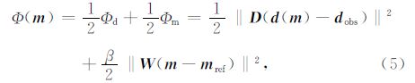
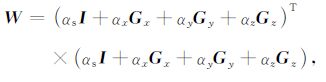
一般采用加上模型约束的正则化方法,变成无约束的最优化问题,其目标泛函为:
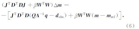
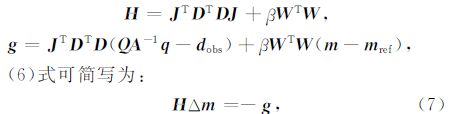
Gauss-Newton方法的法方程形式为:
Haber等(2000)将J表示为:

(1)先计算一个中间向量w=Bv;
(2)然后求解线性系统y=A-1w;
(3)之后y向量左乘投影矩阵Q即可.
由于反演过程中需要反复求解三维正演的线性系统y=A-1w来完成雅可比矩阵与向量的乘积,因而求解Gauss-Newton反演的法方程非常耗时.同样基于不完全Gauss-Newton思想,在计算矩阵向量积Hv时,设置较低的正演计算精度.JTv的计算类似,详见相关文献(吴小平和徐果明,1999;李长伟等,2012),大大提高了电阻率三维不完全Gauss-Newton反演算法的效率.
引入上述方法之后,简要的不完全Gauss-Newton反演流程如下:
(1)给定初始模型和参考模型,均取为均匀半空间.
(2)利用PCG算法不精确求解方程(7),获得模型修正量Δm.
(3)确定线性搜索步长α:
α初始值为1,子迭代中,每次迭代使α减小(Armijo,1966),本文中每次线性搜索迭代使α变为之前的一半,直到满足目标函数优化:

(4)更新模型:
(5)判断是否继续迭代:
计算目标函数并估计数据残差,若满足精度要求则反演结束并输出结果;若不满足,重复步骤(2)—(4)进行迭代.对于节点数为250000左右的非结构网格,约5次迭代可得到较好的结果,总迭代次数一般不超过10次.反演程序由Intel Fortran编译运行,在PC上计算耗时30 min左右(CPU为i5-3.2 GHz,内存为8 G).
4 任意偶极-偶极数据的电阻率三维反演 4.1 任意偶极-偶极观测方式
地表测区为80m×80m,相邻电极间距离均为4m,即地表有21×21个电极测网.取16组AB作为供电偶极:对于测区80m×80m的正方形,有4组AB为其4条边(AB=80m),2组AB为其对角边(AB=80 m),另2组AB为过中心点的正交中线(AB=80m),共8组供电AB极;为了进一步增强探测深度,对于测区外围的160m×160m的正方形,也以同样方式取8组供电AB,AB分别为160m、160m、160m.以上所述观测装置如图 7所示,其中源点用红点表示,测点用蓝点表示.针对每组供电AB,在测量电极中随机选取100组MN观测电极组合,即每次随机取两个蓝点的电位差计算视电阻率,共形成1600组视电阻率观测数据,用于以下各个模型的反演实验.
 |
图 7 随机观测装置示意图 Fig. 7 Schematic of the r and om acquisition |
实际上,由于非结构网格单元的建模优势,可以针对不同地形特点,设计该地形条件下最合理的观测方式,即对任意形式的偶极-偶极测量数据,无论观测方式简单或复杂,均可用于本文任意地形条件下的三维电阻率反演.
4.2 平坦地形下高阻体模型的反演模型设置如前文图 3中模型,即平坦地形下有一立方体高阻异常,背景电阻率为200 Ωm,异常体电阻率为2000 Ωm.反演结果如图 8所示,该结果表 明地下存在高阻异常,与图 3所示的模型示意图相 当一致,定位准确,反演获得很好的效果.
 |
图 8 高阻体模型的反演结果 Fig. 8 Inversion of the high resistivity model |
为了验证反演算法的正确性与分辨率,反演更为复杂一些的模型很有必要.图 9为平坦地形下并排两个立方体异常模型,其中一个为低阻体,电阻率20 Ωm;另一个为高阻体,电阻率2000 Ωm,顶部埋 深均为10 m,异常间隔20 m,背景电阻率为200 Ωm.
 |
图 9 低阻和高阻共存的组合模型示意图 Fig. 9 Schematic diagram of the model with low and high resistivity anomalous bodies |
反演结果如图 10所示,清楚地反映了地下低阻与高阻异常体并存,横向分辨率很好,并且没有其他的多余结构会影响解释结果.与图 9所示的真实模型示意图相比,定位准确,吻合好,反演结果很好地分辨了地下真实的电性结构.
 |
图 10 低阻和高阻异常体的组合模型反演结果 Fig. 10 Inversion of the combination model with a low resistivity and a high resistivity anomalous bodies |
模型设置如前文图 5中模型,山峰地形下有一立方体高阻异常,背景电阻率为200 Ωm,异常体电阻率为2000 Ωm.倘若不考虑山峰地形的影响,直接使用平坦地形下的电阻率三维反演,则结果如图 11所示,显示地下为一低阻异常体,与图 5的真实模型完全不一致.可见,地形造成的影响非常大,甚至获得相反的异常结果.
 |
图 11 山峰地形下高阻体模型的反演结果,反演中没有考虑地形 Fig. 11 Inversion of the high resistivity model under a hill,ignoring the influence of the topography |
吴小平(2005)的结果表明,无论是在数据空间还是在模型空间进行地形校正,起伏地形条件下的电阻率三维反演均不能完全消除地形影响,必须在反演中直接引入地形信息,进行带地形的电阻率三维反演才有可能.图 12为该模型的带地形电阻率三维反演结果,清晰地反映了山峰地形下的高阻异常体,与图 5的真实模型相当一致,有效地消除了地形影响.
 |
图 12 山峰地形下高阻体模型的带地形反演结果 Fig. 12 Inversion of the high resistivity model under a hill, considering the influence of the topography |
实际野外勘察工作中,山峰、山谷起伏不定,地形条件十分复杂.随着GPS/GNSS技术的日益成熟,复杂环境中观测点的准确定位变得简单易行,为灵活、高效的野外电阻率三维测量创造了有利条件.
结合本文实现的任意偶极-偶极视电阻率观测数据的带地形三维反演,将在野外实际数据的三维反演解释中发挥重要作用.
图 13是模拟野外实际情况构建的一个相对复杂的起伏地形及其非结构网格剖分.我们分别反演该复杂地形下的低阻异常体和高阻异常体三维模型,低阻异常体电阻率为20 Ωm,高阻异常体电阻率为2000 Ωm,背景电阻率均为200 Ωm,其他模型参数见图 3.当起伏地形下分别存在低阻异常体和高阻异常体时,带地形电阻率三维反演结果见图 14、图 15,均清晰地反映了地下的真实电阻率结构,获得很好的反演效果,表明本文基于非结构网格的电阻率三维反演方法在野外复杂地形条件下亦可获得可靠结果.
 |
图 13 复杂起伏地形的非结构网格剖分示意图 Fig. 13 Unstructured grids of a complex topography |
 |
图 14 复杂起伏地形下存在低阻异常体的带地形反演结果 Fig. 14 Inversion of the low resistivity model under a complex topography,considering the influence of the topography |
 |
图 15 复杂起伏地形下存在高阻异常体的带地形反演结果 Fig. 15 Inversion of the high resistivity model under a complex topography,considering the influence of the topography |
模型设置与4.2节相同,即平坦地形下有一立方体高阻异常,背景电阻率为200 Ωm,异常体电阻率为2000 Ωm.在生成合成数据时,将默认引入的5%高斯噪声增加为10%高斯噪声.反演结果如图 16所示,同样取得较好的反演结果,电阻率结构清晰并且无多余的虚假信息.与图 8的反演结果相比,只是在高阻异常中心处的电阻率值略有减小,表明 本文的电阻率三维反演结果可靠,反演方法对观测数据的噪声依赖性不大.
 |
图 16 引入10%测量误差时高阻体模型的反演结果 Fig. 16 Inversion of the high resistivity model with a measurement error of 10% |
随着GPS/GNSS技术的日益成熟,野外区域地球物理调查中观测点的准确定位变得简单易行,为灵活、高效的野外电阻率三维测量创造了有利条件.结合电阻率三维非结构有限单元数值模拟,本文实现了任意偶极-偶极视电阻率观测数据的带地形三维反演,理论模型反演以及模拟野外实际地形的复杂模型反演均取得很好的效果,模拟实际数据带高斯噪声的三维反演也取得可靠的结果,将对野外实际数据的三维反演解释向前推进关键一步.
| [1] | Armijo L. 1966. Minimization of functions having Lipschitz continuous first partial derivatives. Pac. J. Math., 16(1):1-3. |
| [2] | Bentley L R, Gharibi M. 2004. Two-and three-dimensional electrical resistivity imaging at aheterogeneous remediation site. Geophysics, 69(3):674-680. |
| [3] | Chambers J E, Ogilvy R D, Kuras O, et al. 2002. 3D electrical imaging of known targets at a controlled environmental test site. Environ. Geol.,41(6):690-704. |
| [4] | Chambers J E, Wilkinson P B, Kuras O, et al. 2011. Three-dimensional geophysical anatomy of an active landslide in Lias Groupmudrocks, Cleveland Basin, UK. Geomorphology, 125(4):472-484. |
| [5] | Chen J Y, Dang Y M, Cheng P F. 2007. Development and progress in GNSS. Journal of Geodesy and Geodynamics(in Chinese), 27(5):1-4. |
| [6] | Chen Q L, Hu J H. 1998. The use of portable GPS in electrical prospecting. Geophysical Prospecting for Petroleum(in Chinese), 37(4):128-133. |
| [7] | Dabas M, Tabbagh A, Tabbagh J. 1994. 3-D inversion in subsurface electrical surveying-I. Theory. Geophys. J. Int.,119(3):975-990. |
| [8] | Dai Q W, Chai X C, Chen D P. 2012. 3D DC resistivity inversion based on damped Gauss-Newton method. Chinese Journal of Engineering Geophysics (in Chinese), 9(4):375-379. |
| [9] | Dembo R S, Eisenstat S C, Steihaug T. 1982. Inexact newton methods. SIAM J. Numer. Anal., 19(2):400-408. |
| [10] | Di Q Y, Wang M Y, Yan S M, et al. 1997. The application of the high density resistivity method for the seawave-proof dam in Zhuhai-harbour. Progress in Geophysics(in Chinese), 12(2):79-88. |
| [11] | Fu L K. 1983. Electrical Prospecting Tutorial(in Chinese). Beijing:Geological Publishing House. |
| [12] | Günther T, Rücker C, Spitzer K. 2006. Three-dimensional modelling and inversion of DC resistivity data incorporating topography—II. Inversion. Geophys. J. Int.,166(2):506-517. |
| [13] | Haber E, Ascher U M, Oldenburg D. 2000. On optimization techniques for solving nonlinear inverse problems. Inverse Problems, 16(5):1263-1280. |
| [14] | Haber E. 2005. Quasi-newton methods for large-scale electromagnetic inverse problems.Inverse Problems, 21(1):305-323. |
| [15] | He J S. 1997. Development and prospect of electrical prospecting method. Chinese J.Geophys.(Acta Geophysica Sinica)(in Chinese), 40(S1):308-316. |
| [16] | Holcombe H T, Jiracek G R. 1984. Three-dimensional terrain corrections in resistivity surveys. Geophysics, 49(4):439-452. |
| [17] | Huang J G, Ruan B Y, Bao G S. 2004. Resistivity inversion on 3-D section based on FEM. Journal of Central South University(Science and Technology)(in Chinese), 35(2):295-299. |
| [18] | Kneisel C, Emmert A, Kstl J. 2014. Application of 3D electrical resistivity imaging for mapping frozen ground conditions exemplified by three case studies. Geomorphology, 210:71-82. |
| [19] | Large D B. 1971. Electric potential near a spherical body in a conducting half-space. Geophysics, 36(4):763-767. |
| [20] | Li C W, Xiong B, Wang Y X, et al. 2012. Inversion of IP logging based on improved Krylov subspace methods. Chinese J.Geophys.(in Chinese), 55(11):3862-3869, doi:10.6038/j.issn.0001-5733.2012.11.034. |
| [21] | Li G F, Yan X L. 2010. Positioning accuracy test of portable GPS receiver and its application in geological exploration of mineral. Geotechnical Engineering World(in Chinese), 1(4):380-384. |
| [22] | Li Y G, Oldenburg D W. 1994. Inversion of 3-D DC resistivity data using an approximate inverse mapping. Geophys. J. Int.,116(3):527-537. |
| [23] | Li Y G, Spitzer K. 2002. Three-dimensional DC resistivity forward modelling using finite elements in comparison with finite-difference solutions. Geophys. J. Int.,151(3):924-934. |
| [24] | Lin J, Shi L. 1996. Prospect for application of GPS survey in geophysical exploring. Equipment for Earth Science(in Chinese), 4:1-5. |
| [25] | Liu B, Li S C, Li S C, et al. 2012a. 3D electrical resistivity inversion with least-squares method based on inequality constraint and its computation efficiency optimization. Chinese J.Geophys.(in Chinese), 55(1):260-268, doi:10.6038/j.issn.0001-5733.2012.01.025. |
| [26] | Liu B, Nie L C, Li S C, et al. 2012b. 3D electrical resistivity inversion tomography with spatial structural constraint. Chinese Journal of Rock Mechanics and Engineering(in Chinese), 31(11):2258-2268. |
| [27] | Liu H M, Zhao H. 2013. The use of portable GPS in electrical and magnetic prospecting for network layout. West-China Exploration Engineering(in Chinese), 25(8):86-88. |
| [28] | Liu S J, Song Z C, Liu G. 2006. Error analysis of handheld GPS positioning in field geological survey. Surveying and Mapping of Sichuan (in Chinese), 29(1):11-14. |
| [29] | Loke M H, Barker R D. 1996. Practical techniques for 3D resistivity surveys and data inversion. Geophysical Prospecting, 44(3):499-523. |
| [30] | Lu J J, Wu X P, Spitzer K. 2010. Algebraic multigrid method for 3D DC resistivity modelling. Chinese J. Geophys.,53(3):700-707. |
| [31] | Oppliger G L. 1984. Three-dimensional terrain corrections for mise-à-la-masse and magnetometric resistivity surveys. Geophysics, 49(10):1718-1729. |
| [32] | Pan K J, Tang J T. 2014. 2. 5-D and 3-D DC resistivity modelling using an extrapolation cascadic multigrid method. Geophys. J. Int., 197(3):1459-1470. |
| [33] | Papadopoulos N G, Tsourlos P, Tsokas G N, et al. 2006. Two-dimensional and three-dimensional resistivity imaging in archaeological site investigation. Archaeol. Prospect.,13(3):163-181. |
| [34] | Papadopoulos N G, Tsourlos P, Tsokas G N, et al. 2007. Efficient ERT measuring and inversion strategies for 3D imaging of buried antiquities. Near Surf. Geophys.,5(6):349-361. |
| [35] | Park S K, Van Gregory P. 1991. Inversion of pole-pole data for 3-D resistivity structure beneath arrays of electrodes. Geophysics, 56(7):951-960. |
| [36] | Park S. 1998. Fluid migration in the vadose zone from 3-D inversion of resistivity monitoring data. Geophysics, 63(1):41-51. |
| [37] | Pidlisecky A, Haber E, Knight R. 2007. RESINVM3D:A 3D resistivity inversion package. Geophysics, 72(2):H1-H10. |
| [38] | Ren Z Y, Tang J T. 2010. 3D direct current resistivity modeling with unstructured mesh by adaptive finite-element method. Geophysics, 75(1):H7-H17. |
| [39] | Ren Z Y, Tang J T. 2014. A goal-oriented adaptive finite-element approach for multi-electrode resistivity system. Geophys. J. Int.,199(1):136-145. |
| [40] | Rődder T, Kneisel C. 2012. Permafrost mapping using quasi-3D resistivity imaging,Murtèl,Swiss Alps. Near Surface Geophysics, 10(2):117-127. |
| [41] | Rücker C, Günther T, Spitzer K. 2006. Three-dimensional modelling and inversion of dc resistivity data incorporating topography—I. Modelling. Geophys. J. Int.,166(2):495-505. |
| [42] | Sasaki Y. 1994. 3-D resistivity inversion using the finite-element method. Geophysics, 59(12):1839-1848. |
| [43] | Spitzer K. 1995. A 3-D finite-difference algorithm for DC resistivity modelling using conjugate gradient methods. Geophys. J. Int.,123(3):903-914. |
| [44] | Tikhonov A N, Arsenin V A. 1977. Solutions of Ill-posed Problems. Washington:W. H. Winston and Sons. |
| [45] | Tsourlos P I, Szymanski J E, Tsokas G N. 1999. The effect of terrain topography on commonly used resistivity arrays. Geophysics, 64(5):1357-1363. |
| [46] | Wan X L, Xi D Y, Gao E G, et al. 2005. 3-D resistivity inversion by the least-squares QR factorization method under improved smoothness constraint condition. Chinese J. Geophys. (in Chinese), 48(2):439-444, doi:10.3321/j.issn:0001-5733.2005.02.030. |
| [47] | Wang K X, Li F Y, Liu H L, et al. 2012. Handheld GPS positioning accuracy and error. GNSS World of China (in Chinese), 36(6):83-86. |
| [48] | Wang W, Wu X P, Spitzer K. 2013. Three-dimensional DC anisotropic resistivity modelling using finite elements on unstructured grids. Geophys. J. Int.,193(2):734-746. |
| [49] | Weller A, Frangos W, Seichter M. 1999. Three-dimensional inversion of induced polarization data from simulated waste. J. Appl. Geophys., 41(1):31-47. |
| [50] | Wu X P, Xu G M. 1999. Derivation and analysis of partial derivative matrix in resistivity 3-D inversion. Oil Geophysical Prospecting(in Chinese), 34(4):363-372. |
| [51] | Wu X P, Xu G M. 2000. Study on 3-D resistivity inversion using conjugate gradient method. Chinese J.Geophys.(in Chinese), 43(3):420-427, doi:10.3321/j.issn:0001-5733.2000.03.016. |
| [52] | Wu X P, Wang T T. 2002. Progress of study on 3D resistivity inversion methods. Progress in Geophysics(in Chinese), 17(1):156-162, doi:10.3969/j.issn.1004-2903.2002.01.023. |
| [53] | Wu X P. 2003. A 3-D finite-element algorithm for DC resistivity modelling using the shifted incomplete Cholesky conjugate gradient method. Geophys. J. Int.,154(3):947-956. |
| [54] | Wu X P, Xiao Y F, Qi C, et al. 2003. Computations of secondary potential for 3D DC resistivity modelling using an incomplete Choleski conjugate-gradient method. Geophysical Prospecting, 51(6):567-577. |
| [55] | Wu X P. 2005. 3-D resistivity inversion under the condition of uneven terrain. Chinese J.Geophys.(in Chinese), 48(4):932-936, doi:10.3321/j.issn:0001-5733.2005.04.028. |
| [56] | Yang Y X. 2010. Progress, contribution and challenges of compass/Beidou satellite navigation system. Acta Geodaetica et Cartographica Sinica(in Chinese), 39(1):1-6. |
| [57] | Yi M J, Kim J H, Song Y, et al. 2001. Three-dimensional imaging of subsurface structures using resistivity data. Geophysical Prospecting, 49(4):483-497. |
| [58] | Zhang J, Mackie R L, Madden T R. 1995. 3-Dresistivity forward modeling and inversion using conjugate gradients. Geophysics, 60(5):1313-1325. |
| [59] | Zhdanov M S, Keller G V. 1994. The Geo-Electrical Methods in Geophysical Exploration(Vol. 31). Netherlands:Elsevier Science Limited. |
| [60] | Zhou B, Greenhalgh S A. 2001. Finite element three-dimensional direct current resistivity modelling:accuracy and efficiency considerations. Geophys. J. Int.,145(3):679-688. |
| [61] | 陈俊勇, 党亚明, 程鹏飞.2007.全球导航卫星系统的进展.大地测量与地球动力学, 27(5):14. |
| [62] | 陈清礼, 胡家华.1998.手持式GPS在电法勘探中的应用.石油物探, 37(4):128-133. |
| [63] | 戴前伟, 柴新朝, 陈德鹏.2012.基于阻尼型高斯牛顿法的三维直流电阻率反演.工程地球物理学报, 9(4):375-379. |
| [64] | 底青云, 王妙月, 严寿民等.1997.高密度电阻率法在珠海某防波堤工程中的应用.地球物理学进展, 12(2):79-88. |
| [65] | 傅良魁.1983.电法勘探教程.北京: 地质出版社. |
| [66] | 何继善.1997.电法勘探的发展和展望.地球物理学报, 40(增刊):308-316. |
| [67] | 黄俊革, 阮百尧, 鲍光淑.2004.基于有限单元法的三维地电断面电阻率反演.中南大学学报(自然科学版),35(2):295-299. |
| [68] | 李长伟, 熊彬, 王有学等.2012.基于改进Krylov子空间算法的井中激电反演.地球物理学报, 55(11):3862-3869,doi:10.6038/j.issn.0001 5733. |
| [69] | 李国防, 闫新亮.2010.手持GPS定位精度测试及其在矿产勘查中的应用.矿产勘查, 1(4):380-384.2012.11.034. |
| [70] | 林君, 石磊.1996.GPS在地球物理勘探中的应用展望.地学仪器, 4:1 5. |
| [71] | 刘斌, 李术才, 李树忱等.2012a.基于不等式约束的最小二乘法三维电阻率反演及其算法优化.地球物理学报, 55(1):260-268,doi:10.6038/j.issn.0001 5733. |
| [72] | 刘斌, 聂利超, 李术才等.2012b.三维电阻率空间结构约束反演成像方法.岩石力学与工程学报, 31(11):2258-2268.2012.01.025. |
| [73] | 刘会敏, 赵灏.2013.手持GPS在电、磁法勘探测网布设工作中的应用.西部探矿工程, 25(8):86-88. |
| [74] | 刘少杰, 宋在超, 刘刚.2006.野外地质测量中手持GPS定位的误差分析.四川测绘, 29(1):11-14. |
| [75] | 宛新林, 席道瑛, 高尔根等.2005.用改进的光滑约束最小二乘正交分解法实现电阻率三维反演.地球物理学报, 48(2):439-444,doi:10.3321/j.issn:0001 5733.2005.02.030. |
| [76] | 王克晓, 李凤友, 刘焕玲等.2012.手持GPS定位精度与误差的研究.全球定位系统, 36(6):83-86. |
| [77] | 吴小平, 徐果明.1999.电阻率三维反演中偏导数矩阵的求取与分析.石油地球物理勘探, 34(4):363-372. |
| [78] | 吴小平, 徐果明.2000.利用共轭梯度法的电阻率三维反演研究.地球物理学报, 43(3):420-427,doi:10.3321/j.issn:0001 5733.2000.03.016. |
| [79] | 吴小平, 汪彤彤.2002.电阻率三维反演方法研究进展.地球物理学进展, 17(1):156-162,doi:10.3969/j.issn.1004 2903. |
| [80] | 吴小平.2005.非平坦地形条件下电阻率三维反演.地球物理学报, 48(4):932-936,doi:10.3321/j.issn:0001 5733.2002.01.023. |
| [81] | 杨元喜.2010.北斗卫星导航系统的进展、贡献与挑战.测绘学报, 39(1):1 6.2005.04.028. |