 2015, Vol. 58


2. 中国科学院大学, 北京 100049
2. University of Chinese Academy of Sciences, Beijing 100049, China
The OH airglow emission spectra were observed by the ground-based spectrometer from December 2011 to December 2013. The OH(8-3) band is used to calculate rotational temperature. The temperatures from SABER are weighted vertically by the weighting functions from its OH-A channel volume emission rates. Firstly, the rotational temperature is compared with the SABER. Secondly, the daily mean temperatures are fitted by the harmonic waves, and the temporal variation features during nights are analyzed.
The comparison between OH rotational temperature and SABER shows that the mean rotational temperature of OH(8-3) band is 203.0±11.2 K with 5.5 K warmer than SABER's. Both have obviously identical seasonal variations and the temperature variation of winter to summer can reach 60 K. The annual and semiannual components are the two most significant variations, and the annual amplitude of 10.8 K is greater than semiannual amplitude of 2.7 K. Their phases are respectively in December and March. It is shown that there are multiple temporal rotational variations during night, such as oscillations controlled by tides and short-period waves.
The OH rotational temperature is a good proxy for the kinetic temperature in the MLT region. There are significant annual and semiannual variations in this region, and the temperatures during night have various temporal features. It is concluded that the temporal variations of ground-based rotational temperatures from OH(8-3) band are well correlated with the SABER temperatures. They have the same seasonal variations and the annual and semiannual oscillations are the two strongest components. The nocturnal rotational temperatures have multiple temporal features controlled by the various oscillations.
中层顶低热层区域的OH气辉辐射,主要由臭氧和氢的化学反应产生,其位于约87 km高度附近,厚约8 km的薄层.在OH层的高度上,大气密度还是比较的高,有足够的碰撞使相对低转动能级处于局部热力学平衡状态(Sivjee and Hamwey, 1987; Perminov and Semenov, 1992; Pendleton et al., 1993),所以转动温度与周围环境的动力学温度相等.由光谱观测的OH气辉辐射强度和转动温度广泛地应用于高层大气的化学和动力学研究(Fiocco et al., 1970; Abreu and Yee, 1989; Bittner et al., 2000,2002; Dewan et al., 1992; Dyrl and et al., 2010; French et al., 2000; French and Mulligan, 2010; French and Klekociuk, 2011; 高红,2008).
地基和卫星的遥感是OH气辉辐射最为有效的探测手段. 其中,地基的观测可以对某一区域进行长期、高时间分辨率的研究,而卫星则可以给出全球的分布和变化.其中地基观测相对低廉费用,而又能给出比较好的观测结果,因此不同的地基观测技术在全球范围内被广泛采用(Oberheide et al., 2006; López-González et al., 2007; Smith et al., 2010).通过对地基与卫星观测比较,可以对地面观测可靠性进行验证,从而利用地面连续长期的探测研究某一固定区域中高层大气随时间的变化特性.
2011年11月,在北京东北约100 km的国家天文台兴隆台站(40.39°N,117.58°E)利用光栅光谱仪组建了一套用于大气辐射探测的系统(Zhu et al., 2012).至2014年,已有完整两年的观测.在中国,这是首次利用地面的光谱仪对OH气辉辐射进行长期的观测.与此同时TIMED卫星上搭载的SABER探测器有大气温度和OH气辉发射率的垂直廓线观测.所以本文对这两种观测进行了比较,并且利用计算的OH转动温度研究中层顶区域温度 的季节变化,得出了转动温度在夜间的不同变化形态. 2 仪器与数据
我们的大气辐射观测系统——大气辐射光谱仪(Spectrometer of Atmospheric Radiation)主要由科研级的单色仪、CCD,以及光路系统和控制软件构 成.单色仪采用Czerny-Turner式结构,焦距550 mm,光栅为1200 gr/mm,闪耀波长500 nm,有很高的光谱分辨率;CCD是1024×256的背照式CCD,单个像元尺寸为26 μm;前置光学系统添加了一个与光谱仪F数相匹配的相机镜头;光线入射狭缝为矩 形,高度固定,宽度为0.25 mm,仪器函数的FWHM(Full Width at Half Maximum)约为0.3 nm;仪器的视场角大约是4.5°×0.17°,对应于87 km高度上面积约7 km×0.3 km.观测位置位于国家天文台兴隆台站(40.39°N,117.58°E),于2011年11月24日投入使用,每天夜晚进行观测,观测谱段包含原子氧的绿线(557.7 nm)和红线(630 nm),原子钠的双 线,OH的8-3、4-0、5-1、9-4、6-2、7-3、8-4、7-3以及3-0 带,波长范围从530 nm至1000 nm,一个循环周期大约是15 min.同时位于同一台站的全天空照相 机,提供了夜间5 min一幅,白天20 min一幅的天空云量图片,可以用来对观测天气的筛选.
本文中利用OH(8-3)带(见图 1)观测计算的转动温度研究中层顶区域的温度的季节性变化.可用观测光谱的挑选原则:(a)谱线相对孤立不受相邻谱线的污染,以及高能宇宙线的影响;(b)避开大气的吸收线波段,特别是水汽和氧气的吸收线;(c)选择无云晴朗的天气;(d)在暑暮期间,虽然太阳已经落到地平线以下,但太阳光依然能够照射到OH层的高度,大气分子就会把太阳光散射到观测视场内,所以要在太阳处于地平线以下10°;(e)要尽量避免月 光的污染,所以要取月亮高度角和月相都很小的情况.
 | 图 1 OH(8-3)带振转光谱(观测于2011年12月24日 18 ∶ 46) Fig.1 Vibration-rotational spectra of OH(8-3)b and (observed at 18 ∶ 46,Dec. 24,2011) |
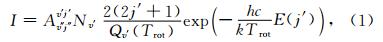
在OH层所在高度上,一般认为分子之间的碰撞频率足够使相对低转动能级的OH分子处于局部热力学平衡状态(Sivjee and Hamwey, 1987),处于某一振动态的OH(v)分子的转动能级服从Boltzmann分布,则谱线的发射强度由以下公式(Mies,1974)给出
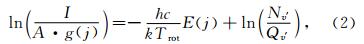
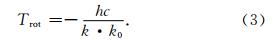
 )和E(j)进行直线拟合出斜率k0,则
所有的观测研究显示(e.g.,Krassovsky et al., 1977; Sivjee and Hamwey, 1987),OH(v)的相对低转动能级基本处于局部热力学平衡状态,所以OH转动能级的布居分布由转动温度唯一确定,并且此转动温度等于周围环境温度. 但是,在计算转动温度时采用的Einstein系数存在误差,导致计算的转动温度与实际大气温度存在差别. French等(2000)和Phillips等(2004)研究了OH(6-2)带和OH(8-3)带的转动温度,结果显示利用LWR(Langhoff,Werner, and Rosmus)(Langhoff et al., 1986)的Einstein 系数计算出的转动温度比利用Mies(Mies,1974)和TL(Turnbull and Lowe, 1989)的Einstein系数计算的转动温度分别低5 K和12 K. 利用LWR Einstein 系数计算的转动温度与实际温度最为接近,因此本文使用此系数.
TIMED(Thermosphere,Ionosphere,Mesosphere,Energetics, and Dynamics)是NASA(National Aeronautics and Space Administration,美国国家航空航天局)于2001年12月发射的一颗中高层大气探测卫星.我们所需要是其上面搭载的SABER(Sounding of the Atmosphere by Broadb and Emission Radiometry)(Russell et al., 1999;Remsberg et al., 2008)version 02.0的Level 2A的温度和OH 发射率的探测数据.SABER临边探测的温度是利用CO2的红外辐射并考虑非局域热力学平衡条件计算得到,在垂直高度上有很高的分辨率,而水平分辨率相对较低,OH气辉发射率的探测有OH-A和OH-B两个通道,波长分别在2.0 μm和1.6 μm,对应的OH的谱带分别是OH(9-7)、OH(8-6)和OH(5-3)、OH(4-2).
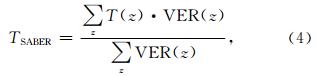
SABER是采用临边观测的方式得到温度的垂直廓线,而地基的OH气辉观测是在垂直高度上的一个积分效应. 不同高度上的气辉强度对于地面观测总强度的贡献正比于OH(v)的分子的密度,所以某一层高度上OH转动温度对地面观测计算得到的转动温度贡献也正比于OH(v)分子密度.因此,地面观测到转动温度是OH层高度上转动温度以OH分子密度分布为权函数的加权等效温度.而OH(v)分子密度随高度的分布可用OH气辉的发射率来代替. 因此在对以上两种观测进行比较时,需要把SABER的温度廓线进行加权平均得到一个等效温度,权函数为OH(v)的分子密度的垂直分布.而SABER的OH发射率观测正好可以用来等效这一权函数.又考虑到不同振动能级的OH分子的垂直分布略有差别,则选择与OH(8-3)相对应的SABER OH-A通道的发射率为权函数,则等效温度为
卫星只是在一天中某几个特定时刻才能到达地基观测的上空,同时考虑水平分辨率不高,选择只要卫星观测点在仪器所在地点经纬度±5°的范围,即可用来进行比较.OH每个谱带循环观测周期约15 min,所以在OH某一谱带观测时间前后7.5 min的SABER观测即可用来比较. 3 结果与分析
根据上面确定地面与卫星的两种观测时空一致标准挑选数据,2012年至2013年OH(8-3)带的平均转动温度为203.0±11.2 K,SABER观测的平均温 度为197.5±10.5 K.与Xiong等(2012)利用SATI4 观测的OH(6-2)带的转动温度在北京天文台(40.30°N,116.19°E)2008年7月至2009年8月的年平均值188±13 K相比,光谱仪观测的OH(8-3)带的转动温度要高. Cosby和Slanger(2007)统计结果显示OH转动温度与振动能级有关,不同振动谱带计算出的转动温度不同.这除了由于不同振动能级OH(v)分子高度分布存在差别外,计算转动温度时,Einstein系数选择对温度计算有很大影响(Cosby and Slanger, 2007).Oberheide等(2006)对OH(3-1)带转动温度与SABER的温度比较显示转动温度要高7.5 K. López-González等(2007)对OH(6-2)带转动温度与SABER温度比较时,转动温度也要高5.7 K. Mulligan和Lowe(2008)对OH(3-1)带转动温度与ACE-FTS,SABER 温度的比较表明地面的转动温度观测要高8.6 K.Smith等(2010)对OH(6-2)带的转动温度与SABER温度比较显示,两者有很好的线性相关性,并且转动温度要比SABER温度高1.7 K.所有地面观测的OH转动温度与卫星观测的温度比较结果都显示,两者存在系统偏差,不过此系统偏差并没有季节性变化.我们的地基观测与SABER观测的比较结果(见图 2)也证实了这一点.因此可以利用转动温度研究中层顶区域温度的相对变化.
 | 图 2 OH(8-3)带转动温度与SABER温度比较 Fig. 2 Comparison of OH(8-3) and SABER temperatures |
从2011年12月至2013年12月总共有效的观测天数为242天.图 3给出了所有有效的OH(8-3)带转动温度随时间的变化.可以看出,转动温度存在非常明显的季节性变化,在夏季5,6月份有温度极小值,冬季11,12月份有温度极大值,在一个夜晚内,转动温度也存在变化,但相较与季节性的波动还是要小得很多.在研究转动温度的季节性变化和年变化时,可以对温度进行日平均处理.由于天气和月光的影响,有时不能整个夜晚都有有效的观测,所以只要这一晚的有效观测数据的累计时间达到4 h,则这一晚即可进行平均来代表这一天的温度.
 | 图 3 OH(8-3)带转动温度(2011年12月至2013年12月) Fig. 3 The rotational temperature of OH(8-3)(From Dec 2011 to Dec 2013) |
在中层顶区域的OH层,年变化和半年变化是两个最强的波动,所以利用地面观测的日平均的转动温度时间序列对这两种波动进行分析,公式如下(Perminov,2009):

 | 图 4 OH(8-3)带的日平均转动温度季节变化以及由公式(5)拟合曲线 Fig. 4 Daily rotational temperature of OH(8-3)b and from Nov 2011 to Dec 2013 and the fitting curve by Eq.(5) |
从计算出的转动温度可以看出,不同夜晚的变化形态不同,但基本上还是有占主导作用的波形变化与Smith等(2010)的观测类似.在中纬度地区,潮汐对于中层顶区域的温度有很强的调制作用,并且一些短周期的重力波叠加在相对长周期的潮汐之上,就会呈现出各种的形态变化.图 5给出了几种典型的计算的转动温度在夜晚随地方时的变化.图 5a显示了8 h潮汐占主导地位时,转动温度的夜晚变化形态,并且振幅可达15 K.图 5b则给出了整个夜晚温度基本保持不变,同时叠加小振幅的波动.图 5c中可以看出,潮汐特征十分显著,同时又有一些短周期的波动叠加其上.图 5d则展示了温度在整个夜晚持续的增加.以上的转动温度夜晚的多样变化形态,反映了中层顶区域存在丰富的动力学过程.
 | 图 5 光谱仪观测不同夜晚转动温度随地方时变化 Fig. 5 Rotational temperatures observed by the spectrometer during nights |
通过安置于中国国家天文台兴隆台站的自主组建的大气辐射观测系统,从2011年12月开始,对 OH气辉辐射进行了连续的观测.利用两年OH(8-3)带光谱的观测计算转动温度,平均温度为203.0±11.2 K. 同时TIMED卫星上SABER探测器有观测点上空的温度剖面观测,其平均温度为197.5±10.5 K.通过两种观测结果比较,OH(8-3)带的转动温度要高于SABER探测温度,不过两者都存在相同的明显的季节变化,夏季有温度极小值,冬季则有温度极大值.通过谐波分析发现,年振荡是最强的波动,振幅达10.8 K,其次半年振荡,振幅则只有2.7 K.年振荡和半年振荡的相位分别在12月初和3月底.
通过地基观测与卫星观测比较,虽然两者存在系统偏差,但这一偏差没有季节性变化,所以地基观测还是可以用于中层顶区域温度的相对变化的研究.下一步工作将利用多谱带的OH气辉辐射研究不同振动态的OH(v)分子高度分布的季节变化,以及利用气辉强度或转动温度研究中层顶区域大尺度的波动,如潮汐、行星波等.
致谢 感谢子午工程数据支持.感谢TIMED/SABER团队提供的卫星探测数据.| [1] | Abreu V J, Yee J H. 1989. Diurnal and seasonal variation of the nighttime OH(8-3) emission at low latitudes. J. Geophys. Res., 94(A9): 11949-11957, doi: 10.1029/JA094iA09p11949. |
| [2] | Bittner M, Offermann D, Graef H H. 2000. Mesopause temperature variability above a midlatitude station in Europe. J. Geophys. Res., 105(D2): 2045-2058, doi: 10.1029/1999jd900307. |
| [3] | Bittner M, Offermann D, Graef H H, et al. 2002. An 18-year time series of OH rotational temperatures and middle atmosphere decadal variations. J. Atmos. Sol. Terr. Phys., 64(8-11): 1147-1166, doi: 10.1016/s1364-6826(02)00065-2. |
| [4] | Cosby P C, Slanger T G. 2007. OH spectroscopy and chemistry investigated with astronomical sky spectra. Can. J. Phys., 85(2): 77-99, doi: 10.1139/p06-088. |
| [5] | Dewan E M, Pendleton W, Grossbard N, et al. 1992. Mesospheric oh airglow temperature fluctuations: A spectral analysis. Geophys. Res. Lett., 19(6): 597-600, doi: 10.1029/92gl00391. |
| [6] | Dyrland M E, Mulligan F J, Hall C M, et al. 2010. Response of OH airglow temperatures to neutral air dynamics at 78°N, 16°E during the anomalous 2003-2004 winter. J. Geophys. Res., 115(D7): D07103, doi: 10.1029/2009jd012726. |
| [7] | Espy P J, Hammond M R. 1995. Atmospheric transmission coefficients for hydroxyl rotational lines used in rotational temperature determinations. J. Quan. Spectrosc. Radiati. Trans., 54(5): 879-889, doi: 10.1016/0022-4073(95)00109-x. |
| [8] | Fiocco G, Visconti G, Congeduti F. 1970. Nocturnal variation of the intensity and rotational temperature of the OH(8,3) band in the airglow. Nature, 228(5276): 1079-1080, doi: 1.01038/2281079a0. |
| [9] | French W J R, Mulligan F J. 2010. Stability of temperatures from TIMED/SABER v1.07(2002—2009) and Aura/MLS v2.2 (2004—2009) compared with OH(6-2) temperatures observed at Davis Station, Antarctica. Atmos. Chem. Phys., 10: 11439-11446, doi: 10.5194/acp-10-11439-2010. |
| [10] | French W J R, Klekociuk A R. 2011. Long-term trends in Antarctic winter hydroxyl temperatures. J. Geophys. Res., 116(D4): D00P09, doi: 10.1029/2011jd015731. |
| [11] | French W J R, Burns G B, Finlayson K, et al. 2000. Hydroxyl (6-2) airglow emission intensity ratios for rotational temperature determination. Ann. Geophys., 18(10): 1293-1303, doi: 10.1007/s00585-000-1293-2. |
| [12] | Gao H. 2008. The study on airglow in middle and upper atmosphere (in Chinese). Beijing: Center for Space and Applied Research, Chinese Academy of Sciences. |
| [13] | Krassovsky V I, Potapov B P, Semenov A I, et al. 1977. On the equilibrium nature of the rotational temperature of hydroxyl airglow. Planet. Space Sci., 25(6): 596-597, doi:10.1016/0032-0633(77)90067-8. |
| [14] | Langhoff S R, Werner H J, Rosmus P. 1986. Theoretical transition-probabilities for the OH Meinel system. J. Mol. Spectrosc., 118(2): 507-529, doi:10.1016/0022-2852(86)90186-4. |
| [15] | López-González M J, García-Comas M, Rodríguez E, et al. 2007. Ground-based mesospheric temperatures at mid-latitude derived from O2 and OH airglow SATI data: Comparison with SABER measurements. J.Atmos.Sol.Terr. Phys., 69(17-18): 2379-2390, doi: 10.1016/j.jastp.2007.07.004. |
| [16] | Mies F H. 1974. Calculated vibrational transition probabilities of OH(X2Π). J. Mol. Spectrosc., 53(2): 150-188, doi: 10.1016/0022-2852(74)90125-8. |
| [17] | Mulligan F, Lowe R. 2008. OH-equivalent temperatures derived from ACE-FTS and SABER temperature profiles—a comparison with OH*(3-1) temperatures from Maynooth (53.2°N, 6.4°W). Ann. Geophys., 26(4): 795-811, doi:10.5194/angeo-26-795-2008. |
| [18] | Oberheide J, Offermann D, Russell J M, et al. 2006. Intercomparison of kinetic temperature from 15 μm CO2 limb emissions and OH*(3,1) rotational temperature in nearly coincident air masses: SABER, GRIPS. Geophys. Res. Lett., 33(14): L14811, doi: 10.1029/2006gl026439. |
| [19] | Pendleton W R Jr, Espy P J, Hammond M R. 1993. Evidence for non-local-thermodynamic-equilibrium rotation in the OH nightglow. J. Geophys. Res., 98(A7): 11567-11579, doi: 10.1029/93ja00740. |
| [20] | Perminov V I. 2009. Seasonal temperature variations near the mesopause according to the hydroxyl emission measurements in Zvenigorod. Geomagn. Aeron., 49(6): 797-804, doi: 10.1134/S0016793207060084. |
| [21] | Perminov V I, Semenov A I. 1992. Nonequilibrium of the rotational temperature of OH bands with high vibrational excitation. Geomagn. Aeron., 32(2): 175-178. |
| [22] | Phillips F, Burns G B, French W J R, et al. 2004. Determining rotational temperatures from the OH(8-3) band, and a comparison with OH(6-2) rotational temperatures at Davis, Antarctica. Ann. Geophys., 22(5): 1549-1561, doi: 10.5194/angeo-22-1549-2004. |
| [23] | Remsberg E E, Marshall B T, Garcia-Comas M, et al. 2008. Assessment of the quality of the Version 1.07 temperature-versus-pressure profiles of the middle atmosphere from TIMED/SABER. J. Geophys. Res., 113(D17): D17101, doi: 10.1029/2008jd010013. |
| [24] | Russell J M, Mlynczak M G, Gordley L L. 1999. Overview of the SABER experiment and preliminary calibration results. Proc. SPIE Int. Soc. Opt. Eng., 3756: 277-288, doi:10.1117/12.366382. |
| [25] | Sivjee G G, Hamwey R M. 1987. Temperature and chemistry of the polar mesopause OH. J. Geophys. Res., 92(A5): 4663-4672, doi: 10.1029/JA092iA05p04663. |
| [26] | Smith S M, Baumgardner J, Mertens C J, et al. 2010. Mesospheric OH temperatures: Simultaneous ground-based and SABER OH measurements over Millstone Hill. Adv. Space Res., 45(2): 239-246, doi: 10.1016/j.asr.2009.09.022. |
| [27] | Tubull D N, Lowe R P. 1989. New hydroxyl transition-probabilities and their importance in airglow studies. Planet. Space Sci., 37(6):723-738, doi:10.1016/0032-0633(89)90042-1. |
| [28] | Xiong J G, Wan W X, Ning B Q, et al. 2012. Seasonal variations of night mesopause temperature in Beijing observed by SATI4. Science China Technological Sciences, 55(5): 1295-1301, doi: 10.1007/s11431-012-4779-8. |
| [29] | Xu J Y, Smith A K, Yuan W, et al. 2007. Global structure and long-term variations of zonal mean temperature observed by TIMED/SABER. J. Geophys. Res., 112(D24): D24106, doi: 10.1029/2007JD008546. |
| [30] | Zhu Y J, Xu J Y, Yuan W, et al. 2012. First experiment of spectrometric observation of hydroxyl emission and rotational temperature in the mesopause in China. Sci. China Technol. Sci., 55(5): 1312-1318, doi: 10.1007/s11431-012-4824-7. |
| [31] | 高红. 2008. 中高层大气气辉辐射研究[博士论文]. 北京:中国科学院研究生院(空间科学与应用研究中心). |