 2015, Vol. 58


2. 国土资源部应用地球物理综合解释理论实验室, 长春 130026
2. Laboratory for Integrated Geophysical Interpretation Theory, Ministry of Land and Resources, Changchun 130026, China
目前在石油地震勘探中主要应用的常规Kirchhoff偏移方法虽然计算速度快,但是由于其基于传统的射线传播理论,在射线焦散区内动力学射线参数Q为0,因此在射线焦散区不能得到有限振幅,且无法到达阴影区,所以常规Kirchhoff偏移方法在这些区域不能很好的成像.而高斯波束在焦散区能够得到有限振幅,且在垂直于中心射线的方向上具有一定宽度,能够覆盖到阴影区,因此其对焦散区和阴影区的成像能有一定程度的改善.
1990年,基于前苏联地球物理学家Babich等和捷克地球物理学家 erven等(1982)对高斯波束的研究工作,Hill(1990)将高斯波束应用到了地震偏移成像中,提出了叠后高斯波束偏移方法,给出了一些偏移中如窗口大小、初始波束宽和慢度间隔等初始参数的选取方法,同时亦给出了在时间域中计算高斯波束叠后深度偏移的计算思路.1992年,Hale(1992)详细对比了Kirchhoff偏移,倾斜叠加偏移和高斯波束偏移三者之间的优势和计算效率,高斯波束偏移在计算效果和计算效率上都是要优于前两者的.2001年,Hill(2001)提出了共偏移距的叠前高斯波束偏移方法,使高斯波束偏移方法可以应用到叠前数据当中,从而提高了计算精度.Nowack等(2003)和Gray(2005)都提出了共炮域的高斯波束叠前偏移方法.2009年,Gray等(2009)给出了真振幅高斯波束偏移的计算方法和公式.2010年,Popov等(2010)给出了基于Kirchhoff偏移计算思想的高斯波束偏移.在Hill方法中的上行波场是通过倾斜叠加后的地震数据乘以接收点对成像点的格林函数的共轭所得到的反向延拓场,而Popvo方法中的上行波场是通过对成像点在所有接收点处的格林函数进行类似Kirchhoff绕射积分而得到的.2010年,Bleistein等(2010)又将实数表示的走时变为复数表示的走时,提出了利用复走时表示的高斯波束计算3D情况下振幅的方法,并且给出了3D情况下计算格林函数的最速下降法公式.2012年,岳玉波等(2012)提出了针对复杂地表条件下的保幅高斯束偏移.2013年,段鹏飞等(2013)给出了TI介质下的角度域高斯波束偏移的实现方法.
上述高斯波束偏移方法的共同点是这些偏移算法都是在频率域下进行的.仅Hill在其1990年的文章中给出了时间域下高斯波束叠后偏移的计算思路,但并未完全给出时间域下高斯波束偏移的公式.本文基于Hill和Gray等人的研究成果,使用复走时代替实走时,进一步对Gray共炮高斯波束偏移成像计算公式进行了推导,通过改变积分次序,使用傅里叶变换和Hilbert变换将频率下的计算转换成时间域下的计算,给出了2D情况下时间域的共炮偏移成像公式.同时利用复杂模型对比了时间域高斯波束偏移同频率域高斯波束偏移和普通射线偏移的计算结果,对比结果表明时间域高斯波束偏移在成像精度上优于普通射线偏移,在效率上优于频率域高斯波束偏移.
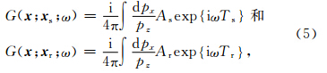
2 时间域高斯波束偏移原理高斯波束叠前偏移是通过高斯波束分别得到源点和接受点在成像点处的格林函数,然后通过这两个格林函数来分别合成下行波场和上行波场,最后通过对下行波场和上行波场做互相关得到成像结果.下面,将从频率域的互相关成像条件来推导出时 间域高斯波束叠前偏移的基本原理,Zhang等(2007)给出了频率域的互相关成像条件为
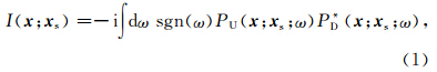
根据Gray等(2009)的文章,用格林函数表示上行波场(地表接收到的反射波场)为
 |
图 1 成像点处的高斯波束偏移示意图Fig. 1 Sketch of Gaussian-beam migration at the image point |
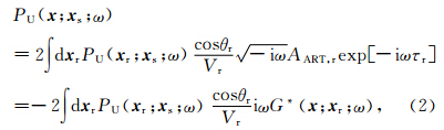
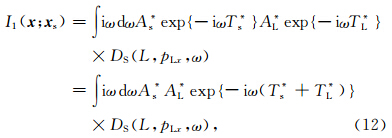
将波场代入到成像函数式(1),得

根据Gray等(2009)中的
 可以得到源点 x s和接收点 x r在成像点 x 处高斯波束表示的格林函数,分别简写为
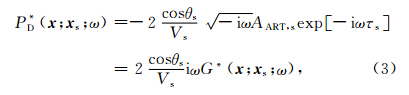
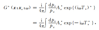
根据e指数的复共轭等于其幂指数的复共轭,可以得到源点 x s和接收点 x r在成像点 x 处高斯波束表示的格林函数的复共轭,分别简写为

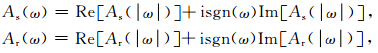
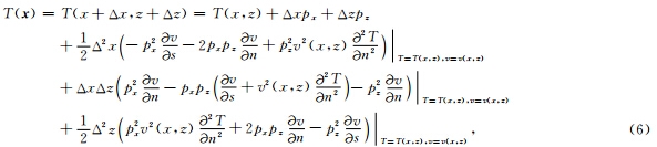
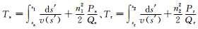 为复数形式所表示的走时,即复走时(Bleistein and Gray, 2010).一般利用距离成像点 x 最近的中心射线上的点 x 0在 x 的二阶泰勒展开来求取 x 处的复走时T(x):
 一般使用公式(6)来求取公式(8)中的Ts和Tr.
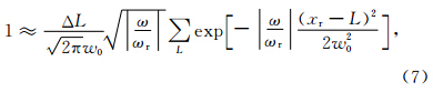
由于高斯波束具有一定宽度,所以接受点处会接收到不同波束的能量,为了区分这些波束,并且将这些波束的能量沿其传播的反方向延拓回去,可以通过倾斜叠加来进行.根据Hill(1990)中的公式
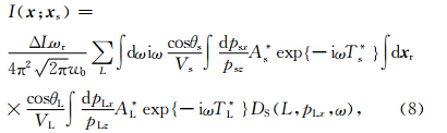
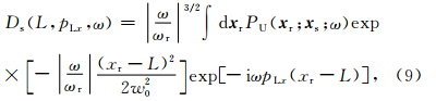
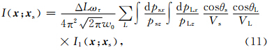
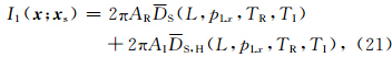
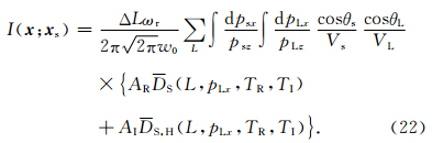
式(8)表示的是先对频率、源点出射的波束和高斯窗中心出射的波束进行三重积分,然后再对不同高斯窗所对应的三重积分求和的过程.对式(8)的三重积分改变积分次序可以得到:
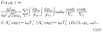
 ×DS(L,pLx,ω)是被积函数,
 是与频率无关的变量.
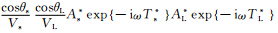
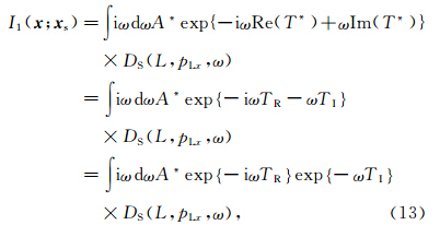
由于最外面两层的积分 是对每一个波束进行的积分,故最内层对频率的积分可以理解为从源点发出的一个波束和接受点发出的一个波束在成像点处的互相关.令:
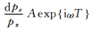
基于Hill(1990)中的公式,可以令
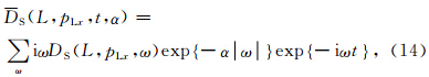
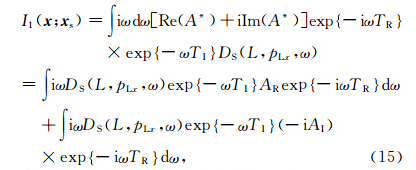
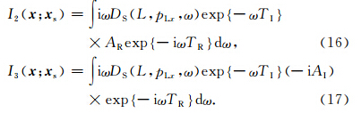
在Hill(Hill,1990)和Aki(Aki and Richards, 1980)的文章和著作中定义傅里叶正变换为∫exp iωt dt,傅里叶反变换为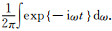 所以基于(14)式,(16)式可表示为

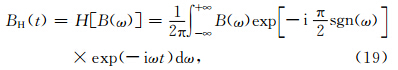
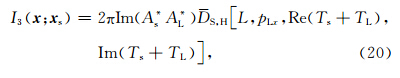
而对式(17),根据Aki等(1980)给出的Hibert变换为
整个程序实现的流程图如图 2.
 |
图 2 偏移方法程序流程图Fig. 2 Flow chart of the program in the migration method |
首先选用Marmousi理论模型数据对时间域高斯波束偏移方法进行检验.图 3a 给出了Marmousi速度模型.Marmousi速度模型横向网格节点数737,横向网格间距12.5 m,长9200 m,纵向网格节点数750,纵向网格间距4 m,深2996 m.图 3b是频率域下高斯波束叠前偏移计算的结果,图 3c是时间域下高斯波束偏移的结果.通过两者对比可以看出频率域下计算结果和时间域下计算结果基本相同,下部背斜构造都能刻画出来,并且上部断层位置也很清晰,和模型所给出的相一致.
 |
图 3(a)Marmousi速度模型,(b)频率域下高斯波束叠前偏移结果,(c)时间域下高斯波束叠前偏移结果Fig. 3(a)Marmousi velocity model.(b)Result of Gaussian beam migration in the frequency domain. (c)Result of Gaussian beam migration in the time domain |
由频率域和时间域两种方法在计算思路上比较可以发现,由于互相关成像条件是一个零时刻的成像条件,在时间域下只需要计算下行波场和上行波场在地震波到达成像点时的值就可以了,而频率域下,必须计算成像点处所有频率所对应的下行波场和上行波场的值,才能通过成像条件得到偏移结果.由于频率域下需要计算多个频率的数据,而时间域只需要计算一个时间点的数据,因此,时间域下的偏 移要比频率域下的偏移更有效率.在图 3的计算过程中,使用的是网上公开的240炮Marmousi模型 模拟数据,每炮96道,时间采样点个数为726,时间 采样间隔为0.004 s,使用的计算机是32位Windows XP 系统,3G主频,4G内存,单核运行.偏移孔径为 以炮点为中心,左右两侧各取长度为最大偏移(2575 m)的矩形孔径.整个地震记录的时间采样长度为726个时间采样点,所以傅里叶变换后对应的零频率和正频率采样点的总个数为364个.在频率域计算过程中需要计算364个频率在成像点处的上下行波场值,而时间域中只需要计算成像时刻在成像点处的上下行波场值就可以了.故而针对Marmousi模型,时间域能够比频率域减少364倍计算上下行波场值的时间.对于Marmousi模型单炮地震记录的偏移时间,频率域为12682 s,时间域为45 s.
选用SMAART JV提供的Sigsbee 2a理论模型和模拟数据对时间域高斯波束偏移方法进行检验.图 4a中给出了Sigsbee 2a速度模型.图 4b是Kirchhoff叠前偏移计算的结果.图 4c是时间域下高斯波束叠前偏移的结果.通过计算结果同模型的对比可以看出Kirchhoff偏移和高斯波束偏移在无高速体覆盖的地层有着良好的成像效果,而在高速体下高斯波束偏移相对于Kirchhoff偏移具有较好的成像效果.在图 4c中白圈内可以看到断层,而在图 4b中的白圈内则出现了更多的偏移假象,看不到清楚的断层.图 4c中的高速体下界面也相对于图 4b中的更清晰.由于文中Kirchhoff偏移是使用波前构建法计算走时表,所以在高速体下方射线稀少的情况可以通过插入新的波前点来改善,而高斯波束偏移则使用由源点出发通过高速体的射线束来成像,故高速体对成像影响较大,造成了在高速体下方高斯波束偏移的能量小于Kirchhoff偏移.
 |
图 4(a)Sigsbee 2a速度模型,(b)Kirchhoff叠前偏移结果,(c)时间域下高斯波束叠前偏移结果Fig. 4(a)Sigsbee 2a velocity model,(b)Result of Prestack Kirchhoff migration in the frequency domain, (c)Result of Prestack Gaussian beam migration in the time domain |
本文中的时间域高斯波束偏移是基于频率域高斯波束偏移推导得到的,通过改变积分次序,引入复走时,将关于频率的积分转化为复走时的函数,从而避免了计算所有频率的格林函数值,节省大量的计算时间.由于时间域高斯波束偏移方法是基于频率域高斯波束偏移方法得到,因此也能够处理多走时的问题,并在焦散区和阴影区取得良好的成像效果.本文研究了构造成像,可为更深入研究时间域高斯波束真振幅成像提供思路和方法.
| [1] | Aki K, Richards P G. 1980. Quantitative Seismology. Staffordshire:Freeman Press. |
| [2] | erven V, Popov M M, Pšeník I. 1982. Computation of wave fields in inhomogeneous media—Gaussian beam approach. Geophysical Journal International, 70(1); 109-128. |
| [3] | Bleistein N, Gray S H. 2010. Amplitude calculations for 3D Gaussian beam migration using complex-valued traveltimes. Inverse Problems, 26(8):085017. |
| [4] | Duan P F, Cheng J B, Chen A P, et al. 2013. Local angle-domain Gaussian beam prestack depth migration in a TI medium. Chinese J. Geophys.(in Chinese), 56(12):4206-4214, doi:10.6038/cjg20131223. |
| [5] | Gray S H. 2005. Gaussian beam migration of common-shot records. Geophysics, 70(4):S71-S77. |
| [6] | Gray S H, Bleistein N. 2009. True-amplitude Gaussian-beam migration. Geophysics, 74(2):S11-S23. |
| [7] | Hill N R. 1990. Gaussian beam migration. Geophysics, 55(11):1416-1428. |
| [8] | Hale D. 1992. Migration by the Kirchhoff, slant stack, and Gaussian beam methods (No. DOE/ER/14079-16; CWP-126). Colorado School of Mines, Golden, CO (United States). Center for Wave Phenomena. |
| [9] | Hill N R. 2001. Prestack Gaussian-beam depth migration. Geophysics, 66(4):1240-1250. |
| [10] | Nowack R L, Sen M K, Stoffa P L. 2003. Gaussian beam migration for sparse common-shot and common-receiver data.//SEG Int. Exposition and 73rd Annual Meeting, 1114-1117. |
| [11] | Popov M M, Semtchenok N M, Popov P M, et al. 2010. Depth migration by the Gaussian beam summation method. Geophysics, 75(2):S81-S93. |
| [12] | Yue Y B, Li Z C, Qian Z P, et al. 2012. Amplitude-preserved Gaussian beam migration under complex topographic conditions. Chinese J. Geophys. (in Chinese), 55(4):1376-1383, doi:10.6038/j.issn.0001-5733.2012.04.033. |
| [13] | Zhang Y, Xu S, Bleistein N, et al. 2007. True-amplitude, angle-domain, common-image gathers from one-way wave-equation migrations. Geophysics, 72(1):S49-S58. |
| [14] | 段鹏飞, 程玖兵, 陈爱萍等. 2013. TI介质局部角度域高斯束叠前深度偏移成像. 地球物理学报, 56(12): 4206-4214, doi: 10.6038/cjg20131223. |
| [15] | 岳玉波, 李振春, 钱忠平等. 2012. 复杂地表条件下保幅高斯束偏移. 地球物理学报, 55(4): 1376-1383, doi: 10.6038/j.issn.0001-5733.2012.04.033. |