 2015, Vol. 58


2. 中国科学院地质与地球物理研究所, 北京 100029;
3. 中国石油西部钻探苏里格气田项目经理部, 鄂尔多斯乌审旗 017300
2. Institute of Geology and Geophysics, Chinese Academy of Sciences, Beijing 100029, China;
3. CNPC Xibu Drilling Engineering Sulige Gas Field Development, Ordos Uxin Qi 017300, China
The method we used to make forward modeling of the gravity anomaly is based on the algorithm proposed by Parker and Oldenburg which uses constant density contrast. We substituted the constant density function in gravity forward formula for the parabolic density function. Then the Fast Fourier Transform (FFT) was applied to both sides of the equation. We derived the gravity anomaly formula of 3D density interface with parabolic density contrast after calculating the involved integral. To invert the density interface depth, an iterative algorithm was preformed to adjust the interface depth step by step until the difference between the theoretical anomalies and observations reduced to the threshold value. In addition, in order to avoid the divergence of the algorithm which is difficult to avoid for the calculation in the frequency domain, we also added a low-pass filter to the codes.
We applied our method to a theoretical model which has 91×71 grid data with 10 km interval in x-axis and y-axis, and a complex 3D interface with parabolic density contrast variation in depth. In the synthetic test, we compared the method proposed in this paper with the constant, exponential and binomial functions. Besides the points with acute topography fluctuation, the results show that the inversion using parabolic function provides good and stable estimates of the interface depth of the theoretical model with RMS 0.02 km, and that the constant density function inversion gives the worst estimate of the theoretical model. According to the comparison, the choice of density parameters is a key factor in interface inversion. For the density of real situation, which varies more rapidly at smaller depth and less rapidly at larger depth, the method provides better approximations to density interface depth. In addition, we applied our method to invert the satellite regional gravity anomaly data with 10 km interval in x-axis and y-axis for the Sichuan-Yunnan region, which has complex geological structures with a large number of major faults, and negative gravity anomalies varying from -540~-90 mGal. We applied the method to invert the Moho depth below this region using reference level 35.5 km and density contrast -0.63 g·cm-3 at the earth surface with attenuation coefficient 0.0018. We compared the result with receiver function from Li et al. (2014) and other geological information. The differences between results of receiver function and our method at most seismic stations are less than 6 km. Therefore the Moho discontinuation derived from this method shows good correlation with the results of receiver function, other prior geophysical and geological information.
Density contrast interface inversion is one of the primary subjects in gravity field research for understanding the earth's interior structure. This work combines the merits of the parabolic density model and the algorithm in the frequency domain, and applies the parabolic density function to the Parker-Oldenburg forward modeling and inversion algorithm. The tests on synthetic data and real data prove the new approach is rapid and effective. By inverting gravity anomaly data using this new approach, we obtained the Moho depth distribution in the Sichuan-Yunnan area, which shows that the Moho interface is shallow in the southeast but deep in the northwest. The Longmen Shan fault zone is a transition zone of the Moho depth ranging from 42 km to 58 km.
1 引言
密度界面反演作为了解地球内部结构的一种重要方法,长期以来都是重力学研究的主要内容.Bott(1960)首次提出采用常密度模型迭代反演盆地底界面深度的方法.其后,为了减少重力反演的多解性,增加反演结果的准确度,Leão等(1996)和Barbosa等(1997)在常密度模型反演基础上加入了深度约束.然而,实际岩石密度是随着地下压力、压实程 度、孔隙度、年龄和深度等因素变化的(Athy,1930). 前人研究表明岩石密度的增加在浅处比深处更快(Cordell,1973),由此可见,变密度函数更符合实际的地质情况.1973年Cordell在沉积盆地的重力异常解释中提出了基于指数模型的界面反演算法.Rao(1986)将二项式密度模型应用于美国加州圣哈辛托盆地的二维重力模拟中也取得了较好的结果.Rao等(1993)研究发现抛物线模型不但能很好地拟合实际密度数据,而且能够近似给出多种地质模型的重力异常表达,并将其应用于圣哈辛托盆地和南亚历桑那州图森盆地的异常解释中,两个地区都取得了很好的反演结果.与二项式模型和指数模型的对比研究表明,抛物线函数能更好地拟合大多数实际地层的密度数据(Rao et al., 1994).Işlk和Şenel(2009)将抛物线密度模型与常密度模型分别应用于土耳其Büyük Menderes盆地的重力异常解释中,两种模型的对比显示,抛物线密度模型反演结果与盆地的实际深度分布更加接近.
在重力界面反演中,除了所用密度函数的不同,根据计算域的不同还可分为空间域反演和频率域反演.空间域反演中,常用的方法是将地下结构分为多个小的单元,然后将这些小单元在地表引起的异常进行叠加,并将叠加结果与实际观测值进行对比.但是,对于复杂的地质体模型和随着地表观测点的增加,运算量急剧加大,运算速度会显著下降.快速傅氏变换(FFT)的发展及其在地学领域中的应用,使得地学数据的处理速度大大加快.Parker(1973)首次将FFT方法引入到位场数据处理中,通过谱展开的方法计算了常密度模型地质体在频率域中的重力场异常.其后,基于Parker公式Oldenburg(1974)提出了位场异常的密度界面迭代反演方法.作为Parker-Oldenburg公式的推广,Guspi(1993)给出了垂向密度分布为多项式时的三维频率域重力异常正反演公式,使得Parker-Oldenburg方法更加普遍化.柯小平等(2006)在青藏高原莫霍面深度反演中应用了指数密度模型的频率域计算并取得了良好的效果.
已有研究(Rao et al., 1993)表明抛物线模型能更好地拟合实际地层密度,而频率域算法又具有快速有效的特点,为此本研究结合了抛物线密度模型及频率域算法的优点,将抛物线密度模型代入Parker-Oldenburg算法,实现了抛物线密度模型的频率域三维界面正反演计算,并通过理论模型数据和实际重力资料反演,验证本方法的正确性和实用性. 2 方法原理 2.1 基于抛物线密度模型的频率域正演计算
基本计算原理如图 1所示,假设界面上下物质的密度分别为ρ1和ρ2,则界面起伏Δh在地表引起的重力异常可由图中阴影部分的剩余质量来计算,此时的剩余密度为σ = ρ1-ρ2.
 | 图 1 密度界面示意图(修改自冯娟等,2014) Fig. 1 Density interface(Modified from Feng et al., 2014) |
假设目标界面之上的密度可用抛物线型密度模型σ(ζ)=σ03/(σ0-αζ)2(Rao et al., 1993)来表示.其中σ(ζ)为深度ζ处的密度差函数,σ0为地表密度差,α为衰减系数.在实际应用中,α的值可由已知的不同深度处密度计算得出.
 | 图 2 异常场源坐标系示意 Fig. 2 Gravity field source coordinate |
下面我们来计算目标界面之上剩余质量引起的重力异常.计算中取右手坐标系,如图 2所示:其中(x,y,0)为观测点位置,dv(ξ,η,ζ)为异常点源,σ(ζ)为源点处密度差.因此观测点(x,y,0)处剩余质量引起重力异常可表示为:


由卷积定理可得:

 ,并将
,并将 在ζ=0处进行泰勒展开得:

将公式(5)对ζ积分,最终求得重力异常的频谱:


求得频率域重力异常后,再对其做反傅里叶变换即可得空间域重力异常. 2.2 界面深度的反演流程
由实测异常给定初始模型(公式(7)),然后对初始模型进行正演计算,将正演计算的理论结果与实测异常进行对比,根据对比误差来调整模型(公式(8)),直到理论结果与实测异常达到设定的误差限.具体反演流程如下:
1)读入界面异常数据、密度参数σ0,α及基准面深度z0,并将异常数据变换到频率域得到F[Δg].
2)根据公式(7)计算界面初始模型Δh(0),其中p=F-1[α2ekz0F[Δg]/(2πG)×f(k)],f(k)为滤波系数.
3)对初始模型Δh(0)进行正演计算得出理论重力异常F[Δg](1).
4)由公式(8)修改初始模型Δh(0)得出修改量Δh, 其中p=F-1[(F[Δg]-F[Δg](1))α2ekz0/(2πG)×f(k)].

5)由Δh(1)=Δh(0)+Δh计算得Δh(1).
6)判断是否达到收敛条件 ≤ε, 若未达到收敛则重复步骤3)—5)直至收敛.
7)若经n次迭代后达到收敛,输出最终界面深度数据h=Δh(n)+z0.
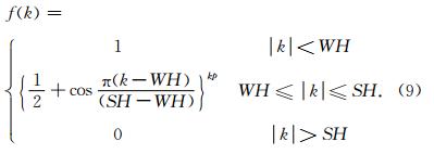
在频率域反演过程中,异常中的高频部分的幅度会随着迭代过程而显著增大,使得程序不容易收敛.因此,在反演计算中我们加入了余弦滤波f(k)(Shin et al., 2006).其原理如式(9)所示.
本文理论密度界面深度范围为34~52 km,如图 3a所示,测网由91×71个测点组成,x、y方向点 距均为10 km.假设密度仅随深度变化,且已知垂向 两点处平均密度差,即h=0 km时,σ0=-0.9 g·cm-3,h=40 km时σ=-0.6 g·cm-3.据此可以得到抛物线密度模型的两个参数(σ0=-0.9 g·cm-3,α=0.0051),与二项式模型(σ(ζ)=σ0+aζ+bζ2)已知参数b=-0.00002时的另外两个参数σ0=-0.9,a=0.0083,以及指数模型((σ(ζ)=σ0eμζ))中参数μ=-0.0101.
 | 图 3 不同密度函数理论模型数据试验反演结果及误差分布 (a)为理论密度界面深度分布,(b)为理论重力异常,(c,e,g,i)分别为常密度模型、 二项式模型、指数模型和抛物线模型反演结果,(d,f,h,j)分别为对应误差分布. Fig. 3 Inversions of the theoretical anomaly and the distribution of the differences between inversions and the theoretical model Theoretical depth of density interface(a) and theoretical gravity anomaly(b). Inverted density interfaces used constant function(c), binomial function(e),exponential function(g) and parabolic function(i) and their corresponding deviations(d,f,h,j). |
图 3b为参考面取z0=40 km时模型正演得到重力异常,异常形态基本与深度分布成反相关,在三个深度极值出现三处重力负异常区.图 3c和3d为 常密度模型(σ=-0.6 g·cm-3)反演结果与误差 分布,图 3e和3f为二项式密度模型(σ=-0.9+0.0083ζ-0.00002ζ2)反演结果与误差分布,图 3g和3h为指数密度模型(σ0=-0.9e-0.0101ζ)反演结果与误差分布,图 3i和3j为抛物线密度模型(σ(ζ)=-0.93/(-0.9-0.0051ζ)2)反演结果与误差分布.在反演中我们取与正演计算时相同的参考面深度 z0=40 km,滤波参数WH=0.05,SH=0.2,kp=5.
对比分析试验结果可以看出,抛物线密度模型 反演结果与理论模型最接近,误差取值范围在-0.5~0.4 km之间,界面深度变化剧烈的地方误差稍大,两者总体均方差为0.02 km,而常密度模型、二项式密度模型、指数密度模型与理论模型的总体均方差分别为0.18、0.04、0.06 km.从图 3中可以看出抛物线模型的反演结果与理论数据间误差最小,除个别深度极值点外,大部分误差在-0.1~0.1 km范围内.常密度模型的反演结果与理论深度相差最大,二项式模型和指数模型效果居中.因此,在进行界面反演过程中合理选取与实际地质体密度分布一致的密 度模型至关重要,否则会在反演结果中引入一定误差. 3.2 川滇地区莫霍面深度反演试验
川滇地区位于青藏高原东南缘,由于受到印度板块对青藏高原推挤作用的影响,发生了强烈的变形和地形反差.区内断层纵横交错,发育了众多深大断裂,如北北西向的哀劳山—红河断裂带、北西向的玉树—甘孜—鲜水河断裂带、近南北走向的安宁河断裂以及北东向龙门山断裂带等,这些断裂作为区内各陆块的边界,对青藏高原东向运动有着重要的调节作用.由于该区所处的特殊大地构造位置和地壳活动的频繁性,长期以来为地质和地球物理学家所重视并在此进行了大量的研究工作(罗志立和龙学明,1992;周荣军等,2006;徐朝繁等,2008;李永华等,2009;姜文亮和张景发,2012;张恩会等,2013).
本文搜集了川滇地区部分岩石物性资料(宋鸿彪和刘树根,1991;Zhang et al., 2010),经最小二乘拟 合得到该区的抛物线密度模型为 σ(ζ)=-0.633/(-0.63-0.0018ζ)2.同时利用地球重力场模型EGM2008(Sandwell and Smith, 2009)计算了该区自由空气重力异常(网度为10 km),然后按照区域重力调查规范作地形校正和布格校正(中间层校正),得到布格重力异常数据(网度为10 km),最终使用优化滤波法(郭良辉等,2012; Guo et al., 2013)分离出川滇地区区域重力异常,作为莫霍面深度重力异常,如图 4所示.校正所用的地形高程数据来自美国斯克里普斯海洋研究所网站(http://topex.ucsd.edu/cgi-bin/get_data.cgi),空间分辨率为1弧分.
 | 图 4 川滇地区区域重力异常 Fig. 4 The gravity anomaly of Moho discontinuities in Sichuan-Yunnan region |
区域重力异常表现为负的重力异常,范围在-90~-540 mGal.汶川—木里—丽江梯级带是区域重力异常的分区带,其东西部场的特征明显不同,反映出地壳性质的明显差异.东部地区异常梯度较大,最高达2 mGal/km左右,西部松潘—甘孜造山带等值线稀疏,变化平缓.
根据前人地球物理探测成果(楼海和王椿镛,2005;楼海等,2010; Teng et al., 2013),反演中参 考面深度取为z0=35.5 km,滤波参数取值为WH=0.01,SH=0.1,kp=1,经过10次迭代反演后,均方差达到0.1 mGal,得到川滇地区莫霍面深度分布(图 5).由图 5可以看出,研究区莫霍面深度介于37.5~66 km之间,其中研究区西北部的松潘—甘孜块体Moho埋深深达~66 km,而四川盆地Moho面埋深最浅,约37.5 km.总体来看,研究区Moho面埋深趋势为东南浅西北深,且在龙门山过渡带上深度变化很快,由西侧松潘—甘孜褶皱带56~66 km降到四川盆地的46~38 km,南部川滇块体与滇西地块下方莫霍面深度40~50 km,与前人采用重力、接收函数方法得到结果(Huang et al., 2002; 钟锴等,2005;黄建平等,2006;Wang et al., 2007;楼海等,2010;Li et al., 2014)基本一致.与Wang 等(2007)H-k叠加分析结果相比,本文在松潘—甘孜地区更加平缓,平均厚度较前者薄3~4 km;与钟锴等(2005)重力异常线性回归法反演相比,本文在攀西地区并无明显上隆.
 | 图 5 采用重力反演得到的川滇地区Moho深度分布及其与接收函数结果的比较(Li et al., 2014) 图中圆点表示地震台站位置,不同颜色代表本文结果减去接收函数结果之差,其中绿色表示误差在-6~6 km, 浅蓝色与黄色分别表示两者相差6~12 km,较大误差用红色与深蓝色表示. Fig. 5 Moho depth distribution of Sichuan-Yunnan region from gravity inversion in this study and comparisons with those from receiver function analysis(Li et al., 2014) Circles give the locations of seismic station. Green circles indicate stations for which the deviations are within ± 6 km. Yellow and light blue circles show stations for which the differences are between 6~12 km. Larger deviations are shown by the red and dark blue circles. |
为了进一步验证反演结果的可靠性,本研究还将上述反演结果与Li等(2014)收集到的地震台站下方接收函数分析结果进行了详细的对比分析,如图 5所示.对比结果显示,63.1%的观测点(178个台站)下方Moho面埋深相差在6 km之内;98.5%的 观测点(275个台站)下方Moho面埋深相差小于12 km; 而二者相差大于12 km的观测点有7个.造成上述不同地球物理方法得到不同Moho面深度的主要原因在于,研究区地壳结构横向变化剧烈,但本研究反演中我们只考虑了密度随深度的垂向变化,而实际上密度在横向上也是变化的. 4 结论
本文结合抛物线密度模型及频率域算法的优点,将抛物线密度函数应用于Parker-Oldenburg界面正反演算法,经过理论推导给出了抛物线密度模型的频率域公式,并编程实现了密度界面的重力异常正反演计算.基于理论模型数据开展的试验研究表明,与常密度模型、二项式密度模型、指数密度模型相比,基于抛物线密度模型的反演结果与理论模型更为接近.
本文还通过反演川滇地区区域重力异常数据,得到了该区莫霍面的深度分布.与传统重力异常反演结果(阚荣举和林中洋,1986;钟锴等,2005)相比,本文方法给出的攀西地区莫霍面深度与人工地震结果(蔡学林等,2007)更为相近,并没有发现莫霍面隆起的现象.通过与接收函数研究结果(Li et al., 2014)进行的对比研究显示,63.1%测点的误差在6 km之内,98.5%测点的误差小于12 km,这也进一步证明了此算法具有良好的反演效果.但由于反演中我们只考虑了密度随深度垂向变化,而未考虑密度在横向上的变化,因此,本文结果与接收函数结果间的大的偏差(>12 km)可能是由横向密度 变化引起的.下一步,我们将考虑以人工地震探测结果作为约束,进行横向密度变化的三维重力界面正反演.
致谢 感谢中国地震局地球物理研究所楼海研究员和中国地质大学(北京)安玉林教授对本文数理推导的耐心指导,感谢中国地质大学(北京)郭良辉副教 授和张盛博士在程序编写过程中提供的帮助,以及 两位匿名评审专家的宝贵建议.| [1] | Athy L F. 1930. Density, porosity, and compaction of sedimentary rocks. AAPG Bulletin, 14(1): 1-24. |
| [2] | Barbosa V C F, Silva J B C, Medeiros W E. 1997. Gravity inversion of basement relief using approximate equality constraints on depths. Geophysics, 62(6): 1745-1757. |
| [3] | Bott M H P. 1960. The use of rapid digital computing methods for direct gravity interpretation of sedimentary basins. Geophysical Journal of the Royal Astronomical Society, 3(1): 63-67. |
| [4] | Cai X L, Zhu J S, Cao J M, et al. 2007. 3D structure and dynamic types of the lithospheric crust in continental China and its adjacent regions. Geology in China (in Chinese), 34(4): 543-557. |
| [5] | Cordell L. 1973. Gravity analysis using an exponential density-depth function—San Jacinto graben, California. Geophysics, 38(4): 684-690. |
| [6] | Feng J, Meng X H, Chen Z X, et al. 2014. The investigation and application of three dimensional density interface. Chinese Journal of Geophysics (in Chinese), 57(1): 287-294, doi: 10.6038/cjg20140124. |
| [7] | Guo L H, Meng X H, Chen Z X, et al. 2013. Preferential filtering for gravity anomaly separation. Computers & Geosciences, 51: 247-254. |
| [8] | Guo L H, Meng X H, Shi L, et al. 2012. Preferential filtering method and its application to Bouguer gravity anomaly of Chinese continent. Chinese Journal of Geophysics (in Chinese), 55(12): 4078-4088, doi: 10.6038/j.issn.0001-5733.2012.12.020. |
| [9] | Guspi F. 1993. Three dimensional Fourier gravity inversion with arbitrary density contrast. Gu X J Trans. Progress in Exploration Geophysics (in Chinese), (5): 39-43. |
| [10] | Huang J L, Zhao D P, Zheng S H. 2002. Lithospheric structure and its relationship to seismic and volcanic activity in southwest China. Journal of Geophysical Research: Solid Earth (1978—2012), 107(B10): ESE 13-1-ESE 13-14. |
| [11] | Huang J P, Fu R S, Xu P, et al. 2006. Inversion of gravity and topography data for the crust thickness of China and its adjacency. Earthquake Science (in Chinese), 28(3): 250-258. |
| [12] | Işlk M, Şenel H. 2009. 3D gravity modeling of Büyük Menderes basin in Western Anatolia using parabolic density function. Journal of Asian Earth Sciences, 34(3): 317-325. |
| [13] | Jiang W L, Zhang J F. 2012. Deep structures of Sichuan-Yunnan region derived from gravity data. Progress in Geophysics (in Chinese), 26(6): 1915-1924, doi: 10.3969/j.issn.1004-2903.2011.06.004. |
| [14] | Kan R J, Lin Z X. 1986. A preliminary study on crustal and upper mantle structures in Yunnan. Earthquake Research in China (in Chinese), 2(4): 50-61. |
| [15] | Ke X P, Wang Y, Xu H Z. 2006. Moho depths inversion of Qinghai Tibet Plateau with variable density model. Geomatics and Information Science of Wuhan University (in Chinese), 31(4): 289-292. |
| [16] | Leão J W D, Menezes P T L, Beltrão J F, et al. 1996. Gravity inversion of basement relief constrained by the knowledge of depth at isolated points. Geophysics, 61(6): 1702-1714. |
| [17] | Li Y H, Wu Q J, Tian X B, et al. 2009. Crustal structure in the Yunnan region determined by modeling receiver functions. Chinese Journal of Geophysics (in Chinese), 52(1): 67-80. |
| [18] | Li Y H, Gao M T, Wu Q J. 2014. Crustal thickness map of the Chinese mainland from teleseismic receiver functions. Tectonophysics, 611: 51-60. |
| [19] | Lou H, Wang C Y. 2005. Wavelet analysis and interpretation of gravity data in Sichuan Yunnan region, China. Acta Seismoligical Sinica (in Chinese), 27(5): 515-523. |
| [20] | Lou H, Wang C Y, Yao Z X, et al. 2010. Subsection feature of the deep structure and material properties of longmenshan fault zone. Earth Science Frontiers (in Chinese), (5): 128-141. |
| [21] | Luo Z L, Long X M. 1992. The uplifting of the Longmenshan orogenic zone and the subsidence of the west Sichuan foreland basin. Acta Geologica Sichuan (in Chinese), 12(1): 1-17. |
| [22] | Oldenburg D W. 1974. Inversion and interpretation of gravity anomalies. Geophysics, 39(4): 526-536. |
| [23] | Parker R L. 1973. The rapid calculation of potential anomalies. Geophysical Journal of the Royal Astronomical Society, 31(4): 447-455. |
| [24] | Rao C V, Chakravarthi V, Raju M L. 1993. Parabolic density function in sedimentary basin modelling. Pure and Applied Geophysics, 140(3): 493-501. |
| [25] | Rao C V, Chakravarthi V, Raju M L. 1994. Forward modeling: Gravity anomalies of two-dimensional bodies of arbitrary shape with hyperbolic and parabolic density functions. Computers & Geosciences, 20(5): 873-880. |
| [26] | Rao D B. 1986. Modelling of sedimentary basins from gravity anomalies with variable density contrast. Geophysical Journal of the Royal Astronomical Society, 84(1): 207-212. |
| [27] | Sandwell D T, Smith W H F. 2009. Global marine gravity from retracked Geosat and ERS-1 altimetry: Ridge segmentation versus spreading rate. Journal of Geophysical Research: Solid Earth (1978—2012), 114(B1), doi: 10.1029/2008JB006008. |
| [28] | Shin Y H, Choi K S, Xu H Z. 2006. Three-dimensional forward and inverse models for gravity fields based on the Fast Fourier Transform. Computers & Geosciences, 32(6): 727-738. |
| [29] | Song H B, Liu S G. 1991. The relation of gravity and aeromagnetic field and deep structure in middle-northern Longmenshan mountains. Journal of Chengdu College of Geology(in Chinese), 18(1): 74-82. |
| [30] | Teng J W, Zhang Z J, Zhang X K, et al. 2013. Investigation of the Moho discontinuity beneath the Chinese mainland using deep seismic sounding profiles. Tectonophysics, 609: 202-216. |
| [31] | Wang C Y, Han W B, Wu J P, et al. 2007. Crustal structure beneath the eastern margin of the Tibetan Plateau and its tectonic implications. Journal of Geophysical Research: Solid Earth (1978—2012), 112(B7), doi: 10.1029/2005JB003873. |
| [32] | Xu Z F, Pan J S, Wang F Y, et al. 2008. Deep geophysical exploration of Longmenshan and its adjacent area. Journal of Geodesy and Geodynamics (in Chinese), 28(6): 31-37. |
| [33] | Zhang E H, Lou H, Jia S, et al. 2013. Characteristics of deep crust structure beneath Western Yunnan. Chinese Journal of Geophysics (in Chinese), 56(3): 252-264, doi: 10.6038/cjg20130614. |
| [34] | Zhang J S, Gao R, Zeng L S, et al. 2010. Relationship between characteristics of gravity and magnetic anomalies and the earthquakes in the Longmenshan range and adjacent areas. Tectonophysics, 491(1-4): 218-229. |
| [35] | Zhong K, Xu M J, Wang L S, et al. 2005. Study on characteristics of gravity field and crustal deformation in Sichuan-Yunnan region. Geological Journal of China Universities (in Chinese), 11(1): 111-117. |
| [36] | Zhou R J, Li Y, Densmore A L, et al. 2006. Active tectonics of the eastern margin of the Tibet plateau. Journal of Mineralogy and Petrology (in Chinese), 26(2): 40-51. |
| [37] | 蔡学林, 朱介寿, 曹家敏等. 2007. 中国大陆及邻区岩石圈地壳三维结构与动力学型式. 中国地质, 34(4): 543-557. |
| [38] | 冯娟, 孟小红, 陈召曦等. 2014. 三维密度界面的正反演研究和应用.地球物理学报, 57(1): 287-294, doi: 10.6038/cjg20140124. |
| [39] | 郭良辉, 孟小红, 石磊等. 2012. 优化滤波方法及其在中国大陆布格重力异常数据处理中的应用. 地球物理学报, 55(12): 4078-4088, doi: 10.6038/j.issn.0001-5733.2012.12.020. |
| [40] | Guspi F. 1993. 任意密度分布的三维傅里叶重力反演. 顾先觉译. 石油物探译丛, (5): 39-43. |
| [41] | 黄建平, 傅容珊, 许萍等. 2006. 利用重力和地形观测反演中国及邻区地壳厚度. 地震学报, 28(3): 250-258. |
| [42] | 姜文亮, 张景发. 2012. 川滇地区重力场与深部结构特征. 地球物理学进展, 26(6): 1915-1924, doi: 10.3969/j.issn.1004-2903.2011.06.004. |
| [43] | 阚荣举, 林中洋. 1986. 云南地壳上地幔构造的初步研究. 中国地震, 2(4): 50-61. |
| [44] | 柯小平, 王勇, 许厚泽. 2006. 用变密度模型反演青藏高原的莫霍面深度. 武汉大学学报 (信息科学版), 31(4): 289-292. |
| [45] | 李永华, 吴庆举, 田小波等. 2009. 用接收函数方法研究云南及其邻区地壳上地幔结构. 地球物理学报, 52(1): 67-80. |
| [46] | 楼海, 王椿镛. 2005. 川滇地区重力异常的小波分解与解释. 地震学报, 27(5): 515-523. |
| [47] | 楼海, 王椿镛, 姚志祥等. 2010. 龙门山断裂带深部构造和物性分布的分段特征. 地学前缘, (5): 128-141. |
| [48] | 罗志立, 龙学明. 1992. 龙门山造山带崛起和川西陆前盆地沉降. 四川地质学报, 12(1): 1-17. |
| [49] | 宋鸿彪, 刘树根. 1991. 龙门山中北段重磁场特征与深部构造的关系. 成都地质学院学报, 18(1): 74-82. |
| [50] | 徐朝繁, 潘纪顺, 王夫运等. 2008. 龙门山及其邻近地区深部地球物理探测. 大地测量与地球动力学, 28(6): 31-37. |
| [51] | 张恩会, 楼海, 嘉世旭等. 2013. 云南西部地壳深部结构特征. 地球物理学报, 56(6): 1915-1927, doi: 10.6038/cjg20130614. |
| [52] | 钟锴, 徐鸣洁, 王良书等. 2005. 川滇地区重力场特征与地壳变形研究. 高校地质学报, 11(1): 111-117. |
| [53] | 周荣军, 李勇, Densmore A L等. 2006. 青藏高原东缘活动构造. 矿物岩石, 26(2): 40-51. |