 2015, Vol. 58

2. 中南大学地球科学与信息物理学院, 长沙 410083
 , FU Hong-Liu1,2, TANG Jing-Tian1,2
 , LIU Feng-Yi1,2, REN Zheng-Yong1,2, YUAN Yuan1,2, ZHANG Lin-Cheng1,2
2. Institute of Geosciences and Info-Physics, Central South University, Changsha 410083, China
The method that this paper adopted is numerical modeling. Based on Maxwell's equations, this paper deduces the impedance formula of planar electromagnetic waves that are obliquely incident on the layered earth under the total current condition in new ways and finishes the corresponding computation programs. The program correctness is verified with comparison to analytic solutions as well as published results. Based on this, the paper calculates and analyzes the apparent resistivity of TE and TM modes varying with displacement currents, incidence angle, magnetic permeability and dielectric permittivity under the quasi-static limit and the total current condition.
According to the various cases of the quasi-static limit and the total current condition, the following information of the relative difference of apparent resistivity of TE and TM modes could be obtained easily. 1) The change of the incidence angle has little impact on TE and TM modes' apparent resistivity under the quasi-static limit. In addition, the apparent resistivity has almost no difference between the two modes. 2) When the incidence angle equals zero, TE and TM modes' apparent resistivity equals each other, which is independent of earth resistivity, frequency, magnetic permeability and dielectric permittivity. As for earth resistivity is above 1000 Ωm, when the incidence angle is below 30 degrees and frequency is less than 1000 kHz, the difference of the apparent resistivity of normally incident and obliquely incident could be ignored. When the incidence angle is greater than 30 degrees and frequency is above 1000 kHz, the difference between the apparent resistivity of normally incident and obliquely incident could not be neglected. At the same time, TE-mode's resistivity increases with the increase of incidence angle, while for TM mode, the opposite holds. Therefore, the difference of the two modes' resistivity increases with increasing incidence angle. Which acts fairly significant especially when frequency is above 1000kHz and incidence angle equals 60 degrees. 3) When the plane electromagnetic wave normally incidents, whether it is under the quasi-static condition, or under the total currents condition, if half-space permeability is not equal to free-space permeability, the calculated apparent resistivity will be μr(μr, the relative permittivity) times of the true half-space resistivity. Under the total currents condition, if the plane electromagnetic wave obliquely incidents on the earth surface, TE-mode's resistivity will be a little smaller than μr times of the true half-space resistivity, while for TM mode, the opposite holds. This is not obvious when frequency is less than 100 kHz, while when frequency is greater than 100 kHz, it acts significantly. 4) As for earth resistivity is greater or equal to 2000 Ωm, the influence of dielectric permittivity on the differences of the two modes' resistivity could be ignored when frequency is less than 100 kHz. While when frequency is greater than 100 kHz, TE or TM-mode's resistivity decreases with the increase of dielectric permittivity. Under the condition of planar electromagnetic wave obliquely incidents, when there is a shallow overburden and frequency equals 1000 kHz, the relative error of the two modes' resistivity maintains 22.5% varying with dielectric permittivity.
In the exploration of the controlled-source audio-frequency magnetotelluric method (CSAMT), if the measured area is not far enough away from the source, it does not meet the planar wave hypothesis, hence the incidence angle should be taken into consideration. In AMT exploration, when the measurement point is located in a high-resistivity geological environment, the apparent resistivity curve of the high frequency section often drops compared to the simulation results under the quasi-static condition, probably because the displacement current cannot be ignored. In the actual exploration, the permeability of the shallow surface has a great influence on the high frequency apparent resistivity, especially when the measurement point is located in the ferromagnetic material. When at higher frequencies or high resistance region, the presence of the dielectric permittivity makes the apparent resistivity decrease. Therefore, in the actual data processing and inversion interpretation, for some special geological condition or at high frequency, the influences of incidence angle, displacement currents, magnetic permeability and dielectric permittivity should be taken into consideration, otherwise we cannot obtain the right conclusions.
在频率小于10 kHz的电磁法勘探中,对大多数地质环境而言,位移电流通常可忽略不计(即准静态假设)(Kaufman and Keller,1987; Nabighian,1992; 李金铭,2005).因此,对于频率较低的电磁勘探方法,一般只需考虑传导电流的作用而忽略位移电流的影响,其处理与解释程序也都不包括位移电流项(Stewart et al.,1994; 林君,2000).但是,当频率较高或在高阻地区,位移电流的影响不可忽略,正反演程序中必须包含位移电流项,否则会出现较大的误差.国内外对位移电流的影响研究始于70年代,主要在航空电磁法(Fraser et al.,1990; Sinha,1997; Huang and Fraser,2002; Yin and Hodges,2005)和高频电磁波探测(朱凯光等,2002a,2002b; 郑圣谈等,2006; 郑圣谈,2007; Kalscheuer et al.,2008; 汤井田等,2009;贺文根等,2013)中研究较多,在音频大地电磁法中则相对较少.
传统的大地电磁法及音频大地电磁法都假设平面电磁波垂直入射地球表面,且忽略位移电流的影响.在准静态条件下,电磁波在空气半空间中的传播常数接近0,远小于地下介质中的波数,因而,无论平面电磁波以何角度入射地球表面,它在大地中总是近似垂直传播(Ward,1971; Song et al.,2002).因此,该情况下,入射角对大地表面的波阻抗基本没有影响.但当位移电流不可忽略时,空气半空间的波数随频率增大而快速增加,电磁波在大地中的传播方向随入射角的不同而有明显改变,入射角对地表波阻抗的影响将逐渐增大,且不可忽略(Poikonen and Suppala,1989).
大地电磁测深法中,一般认为地下介质的介电常数和磁导率与自由空间的相同.由于介电常数对介质的含水量比较敏感,比如,干燥的土壤、灰岩、砂岩本身介电常数不高,但当其中的水含量大时,介电常数值就高.另外,钛锰化合物、方铅矿等金属矿的介电常数也较高(王妙月等,2002).实际地质情况中,还经常遇到超基性侵入岩、含铁石英岩以及其他高磁性体,其磁导率相当大.介电常数和磁导率除影响位移电流的大小外,它们的变化对视电阻也存在影响.某些地质情况下,忽略它们的影响,可能会造成野外资料解释的误差(寇绳武等,1983; Pavlov,2000;黄文彬,2009;习建军,2010).
从查阅的相关文献可知,前人主要研究了位移电流在何种情况下对电磁场响应的影响不可忽略,同时研究了大地电阻率、频率和介电常数等参数对位移电流具有怎样的“贡献”,以及位移电流的存在对电磁场幅值和实虚部分量影响的研究上.而本文则着重于在位移电流不可忽略的情况下,对TE和TM两种模式视电阻率进行对比研究,以及探讨入射角、磁导率和介电常数等参数对两种模式视电阻率差异的影响.
本文从麦克斯韦方程组出发,以新的方式推导了平面电磁波倾斜入射层状介质表面时的波阻抗公式,编制了相应的计算程序,通过与解析解及文献中结果的对比,验证了程序的正确性.在此基础上,分别计算、分析、讨论了准静态极限和全电流条件下电磁波入射角、介电常数和磁导率对TE和TM模式视电阻率之间差别的影响.本文结果既验证了大地电磁法中垂直入射平面电磁波假设的广泛适用性,同时对高频及高阻地质条件下的大地电磁资料分析也具有一定的指导作用.
2 全电流时倾斜入射平面电磁波的阻抗假定平面电磁波以入射角θ0倾斜入射到y-z平面内的n层大地表面上,并且假定x方向为走向方 向,则平面波在空气和大地界面传播情况如图 1所示.

|
图 1 平面波传播示意图 Fig. 1 Schematic diagram of plane wave propagation |
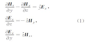
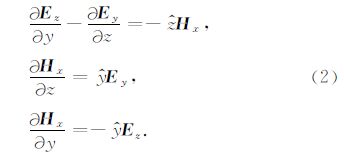
图中σj、μj、εj分别是第j层的电导率、磁导率和介电常数;kj、θj、hj分别是第j层的波数、入射角和层厚; 假定每层电性均匀各向同性,导纳率 y=σ+iωε和电磁场只在y方向和z方向上变化.这种选择定义了TE模式(transverse electric,TE,电场极化 方向平行于地质体走向方向)和TM模式(transverse magnetic,TM,磁场极化方向平行于地质体走向方 向).TE模式和TM模式的方程组分别为(Kalscheuer et al.,2008):
(1)TE-mode:
(2)TM-mode:
在空气和大地中,波数k都有两个方向的分量,分别是水平波数矢量 k y和垂直波数矢量 k z.第j层的传播常数被描述为

其中,ω是角频率;zj=iωμj是阻抗常数; yi=σj+iωεj是导纳率.
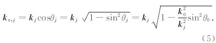
大地表面电磁波的反射和折射由斯奈尔定律和菲涅尔方程决定.水平波数矢量 k y在层状边界上是一个保持不变的常数(Kalscheuer et al.,2008).若第j层的透射角为θj,则有以下关系式:

由方程(3)和(4),可得第j层的垂直波数 k z,j:
假定磁场在入射平面内极化(TE模式),则电场垂直入射平面且有以下形式(Song et al.,2002):

式中,Aj、Bj 分别代表下行和上行平面波电场的振幅.
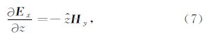
由(6)式和(7)式可得
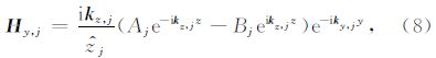
式中 k z,j= k jcosθj,k y,j= k jsinθj.
在层状介质各层之间的边界上,电场和磁场的切向分量是连续的.若z=hi,则
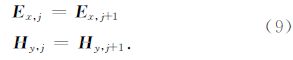
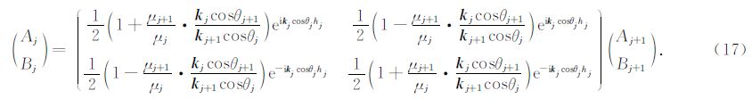
将(6)、(8)两式代入(9)式,经整理并写成矩阵形式可得
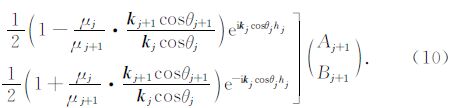
或者
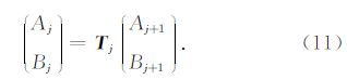
矩阵 T j是第j层的转移矩阵.对于n层模型,可以得到从 T 1到 T n的一个 T j的系列.因此可得递推公式:
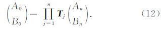
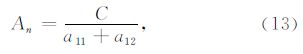
使 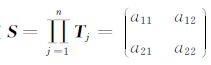 若令地表电场E0=C,又因Bn=0(基底无上行波存在),则可得:
波阻抗的定义(李金铭,2005):
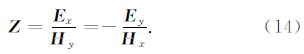
由递推公式(12)式和式(13)可求出第j层的未 知系数Aj和Bj,再结合(14)式,则n层地表波阻抗为
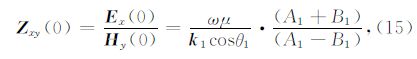
特别的,对于均匀半空间,地表波阻抗为
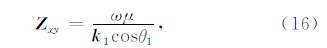
式中, 为第一层中的入射角.
同理,对于TM模式(电场在入射平面内极化),其递推公式为
n层地表波阻抗为

特别的,对于均匀半空间,地表波阻抗为
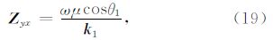
其中,均匀半空间的波阻抗结果同Song等(2002)文献中的结果一致.
卡尼亚视电阻率公式为
利用递推公式和(20)式,可计算全电流时平面电磁波斜入射层状介质表面的视电阻率.
3 计算程序验证根据递推公式和(20)式,编制了全电流条件下平面电磁波倾斜入射层状介质表面的波阻抗和视电阻率计算程序.程序中,相对介电常数设置为0时,即是忽略位移电流时的准静态极限下的计算结果;相对介电常数不为0时,则为全电流下的计算结果.
为验证计算程序的正确性,我们将本文计算结果与解析解及部分文献的结果进行了对比分析.图 2是一个三层模型的计算结果对比,模型参数为 ρ1=100 Ωm,h1=30 m; ρ2=1000 Ωm,h2=300 m; ρ3=10 Ωm. 可以看出,忽略位移电流时,计算结果与准静态条件下的解析解(刘长生,2009)几乎完全一致,最大相对误差为0.00529%,平均相对误差为0.000435%,均方根相对误差为9.02156×10⁻⁶;考虑位移电流时,低频段计算结果与准静态条件下的解析解也是一致的,但计算误差随频率增加而略有增加.这既表明在该模型计算中,准静态假设是可以接受的,同时位移电流对计算精度有一定的影响.

|
图 2 三层模型上计算结果对比 (a)视电阻率曲线;(b)误差曲线.Liu′s曲线是刘长生(2009)给出的结果,Mine曲线是本文的结果.δ为相对误差. Fig. 2 Result comparison of three-layer mode (a)Apparent resistivity curves;(b)Relative error curves. Liu′s curve is the results given by Liu(2009); Mine curve is the results given by this study. |
图 3是本文对Kalscheuer等(2008)文献中一特殊均匀半空间模型(ρ=10000 Ωm)的计算结果.考虑位移电流时,本文结果与Kalscheuer等(2008)给出的结果几乎完全一致.对该模型,是否考虑位移电流,结果显然有比较大的误差,说明在该模型计算中,必须考虑位移电流的影响,否则会带来较大的误差.

|
图 3 均匀半空间模型上计算结果对比(a)视电阻率曲线;(b)误差曲线. Fig. 3 Result comparison of homogeneous mode(a)Apparent resistivity curves;(b)Relative error curves. |
为考察入射角、磁导率和介电常数对大地电磁测深结果的影响,我们绘制了TE、TM模式视电阻率随以上参数的变化曲线,并以准静态极限下垂直入射时的卡尼亚电阻率(此时层状介质的TE、TM模式视电阻率相等)为参考,计算相对误差.分两种情况讨论.
4.1 准静态极限下的结果分析
本节相对误差计算公式为 ,式中ρ*为ρTE或ρTM; ρ为垂直入射时的卡尼亚电阻率.
图 4和图 5分别是均匀半空间和二层介质表面视电阻率曲线和误差图.计算中,磁导率都取自由空间的磁导率.其中均匀半空间情况下,ρTE=ρTM=1000 Ωm,无相对误差.

|
图 4 均匀半空间(ρ=1000 Ωm)视电阻率曲线 (a)频率测深曲线;(b)电阻率随入射角变化曲线. Fig. 4 Apparent resistivity curves of homogeneous half-space(a)Frequency sounding curves;(b)Resistivity curves varied with incident angle. |

|
图 5 二层介质(ρ1=1000 Ωm,h1=100 m;ρ2=2000 Ωm)视电阻率曲线及误差 (a1)频率测深曲线;(a2)误差曲线;(b1)电阻率随入射角变化曲线;(b2)误差曲线. Fig. 5 Apparent resistivity curves and errors of two-layer medium(a1)Frequency sounding curves;(a2)Corresponding relative error curves;(b1)Resistivity curves varied with incident angle; (b2)Corresponding relative error curves. |
图 4和图 5结果表明,在准静态极限下,层状介质表面的TE和TM模式视电阻率几乎相等,且几乎不随平面电磁波入射角而变化,其值都几乎等于垂直入射时的电阻率,这充分说明了大地电磁法基本假设的适用性.同时,从相对误差图可知,电磁波垂直入射时,ρTE=ρTM,无相对误差.频率较低(f<102 Hz)时,入射角对电阻率无影响;频率较高(f>102 Hz)时,入射角对电阻率有影响,且对ρTM影响较ρTE显著,但此时入射角影响仍甚微.这是因为在准静态条件下,方程(5)中 k 0/ k j→0,使得根号下的第二项消失,垂直波数近似等于传播常数本身,即向地下透射的电磁场总是近似垂直传播.
4.1.2 磁导率对视电阻率的影响从均匀半空间表面波阻抗公式(16)、(19)和视电阻率计算公式(20)可知,当半空间磁导率不等于自由空间磁导率时,计算的视电阻率将是半空间真电阻率的μr倍.图 6a的结果直观地印证了该结论. 图 6b是二层介质时的计算结果,第一层磁导率 μ1=(1~5)μ0,第二层磁导率μ2=μ0.图 6c是相同

|
图 6 不同频率下TE、TM模式视电阻率随磁导率的变化(a)均匀半空间(ρ=1000 Ωm);(b)、(c)两层介质(ρ1=1000 Ωm,h1=100 m; ρ2=1000 Ωm);(d)三层介质(ρ1=1000 Ωm,h1=100 m;ρ2=1000 Ωm,h2=100 m;ρ3=1000 Ωm). 其中入射角为θ0=0°,该情况下ρTE=ρTM. Fig. 6 The apparent resistivity of TE or TM mode varies with different magnetic permeabilities under different frequency(a)Homogeneous half-space;(b),(c)Two-layer medium;(d)Three-layer medium. Where the incident angle θ0=0°,under this condition ρTE=ρTM. |
二层模型的计算结果,但第一层和第二层磁导率互换.图 6d是三层介质时的计算结果,它其实是电阻率均匀半空间模型,只是中间层的磁导率不同于自由空间的磁导率,为μ2=(1~5)μ0.对比图 6(a,c)、6(b,d)可知,覆盖层的存在使得磁导率对浅部视电阻率的影响减弱,而磁导率对深部视电阻率的影响几乎不受覆盖层的影响.
在实际勘探中,浅表层的磁导率对高频视电阻率有较大的影响,这种影响主要源于视电阻率计算中采用的是自由空间的磁导率.如果能采用实际地表层的磁导率,将极大地消除这种影响.在野外,虽然磁导率的变化范围很小,基本与自由空间的相同,但对卡尼亚电阻率造成的误差可能会超过观测误差本身,需要加以关注.如果测点恰好位于铁磁性物质上,影响将更大.
4.2 全电流条件当发射频率较高或在特殊的高阻环境下,位移电流的影响变得不可忽略,因而位移电流项在此种情况下必须被考虑到计算程序中.因此,本文在该情况下的正演计算程序考虑全电流情形.在全电流情况下,本文分别研究了入射角、磁导率以及介电常数变化对TE和TM模式视电阻率相对差别的影响.
i4
本节入射角下的相对误差计算公式同准静态下的一样,而磁导率和介电常数下的则为:  .
.
图 7和图 8分别是均匀半空间和二层介质表面视电阻率曲线和误差图.计算中,磁导率都取自由空间的磁导率,即μ1=μ2=μ0,介电常数取ε1=ε2=5ε0.其中μ0=1.256×10⁶ H·m-1,ε0=8.854×10⁻¹²F·m-1.

|
图 7 均匀半空间(ρ=10000 Ωm)视电阻率曲线及误差(a1)频率测深曲线;(a2)误差曲线;(b1)电阻率随入射角变化曲线;(b2)误差曲线. Fig. 7 Apparent resistivity curves and errors of homogeneous half-space(a1)Frequency sounding curves;(a2)Corresponding relative error curves;(b1)Resistivity curves varied with incident angle; (b2)Corresponding relative error curves. |

|
图 8 两层介质(ρ1=2000 Ωm,h1=100 m;ρ2=20000 Ωm)视电阻率曲线及误差(a1)频率测深曲线;(a2)误差曲线;(b1)电阻率随入射角变化曲线;(b2)误差曲线. Fig. 8 Apparent resistivity curves and errors of two-layer medium(a1)Frequency sounding curves;(a2)Corresponding relative error curves;(b1)Resistivity curves varied with incident angle; (b2)Corresponding relative error curves. |
由图 7和图 8中的(a1)、(a2)可知:当入射角 θ0=0°时,ρTE=ρTM,且与频率大小无关.当入射角θ0<30°时,在所研究的频率范围内,δ<5%.当入射角θ0>30°且频率接近106 Hz时,δ>5%.由图 7和图 8中的(b1)、(b2)可知: 当频率f≤105 Hz时,不论入射 角多大,δ<5%;当频率f接近106 Hz且入射角 θ0>30°时,δ>5%.同时,由图 7(a2)和图 8(a2)可知:TE模式视电阻率曲线随入射角的增大而增大,而TM模式视电阻率曲线则正好呈现相反的规律.该规律在频率f≤105 Hz时,表现得不明显,而当频率f=106 Hz时,该规律十分明显.该规律由式(15)、(16)和式(18)、(19)不难解释.由图 7(b2)和图 8(b2)可知:入射角对ρTE影响较ρTM显著.
由以上分析可知:对于同一层状介质模型,当电磁波垂直入射时,TE和TM模式视电阻率相等,与位移电流大小无关.当位移电流大小可忽略不计时,TE和TM模式视电阻率相等,而与入射角无关.当电磁波倾斜入射且位移电流不可忽略时,TE和TM模式视电阻率不再相等,位移电流越大,入射角越大,两者间的差别也越大.当频率f接近106 Hz且入射角θ0>30°时,倾斜入射时的视电阻率同垂直入射时的相比,相对误差δ>5%,且随着入射角的增大而增大.
4.2.2 磁导率变化对TE、TM模式视电阻率的影响图 9和图 10分别为不同磁导率情况下,入射角为θ0=0°、θ0=60°时的视电阻率曲线和误差图.其中各层电阻率都设置为ρi=10000 Ωm,且各层介电常数均取εi=5ε0(i=1,2,3),层厚设置为hi=100 m(i=1,2).除a图中μ、b图中μ1和图(c、d)中μ2皆设置为(1~5)μ0外,其他各层磁导率皆同空气中的磁导率.

|
图 9 不同磁导率下TE、TM模式视电阻率曲线(垂直入射) (a)均匀半空间;(b)、(c)两层介质;(d)三层介质. Fig. 9 Apparent resistivity curves of TE,TM mode among different magnetic permeabilities(normal incident)(a)Homogeneous half-space;(b),(c)Two-layer medium;(d)Three-layer medium. |

|
图 10 不同磁导率下TE、TM模式视电阻率及其相对误差(倾斜入射)(a1)均匀半空间,(a2)相对误差;(b1)、(c1)两层介质,(b2)、(c2)相对误差;(d1)三层介质,(d2)相对误差. Fig. 10 Apparent resistivity curves of TE,TM mode among different magnetic permeabilities(obliquely incident)(a1)Homogeneous half-space;(a2)Corresponding relative error;(b1),(c1)Two-layer medium; (b2),(c2)Corresponding relative error;(d1)Three-layer medium,(d2)Corresponding relative error. |
由图 9可知:当入射角θ0=0°时,ρTE=ρTM,且与 磁导率和频率大小无关.由图 10可知:当入射角 θ0=60°时,ρTE≠ρTM,不过当频率f<105 Hz时,无论磁导率多大,δ<3%.由图 10(a1,b1)可知:TE或TM视电阻率随着磁导率的增加而增加.由图 10(a2,b2)可知:当频率f=106 Hz时,δ>5%,且随着磁导率减小,δ逐渐增大.由图 10(c1,d1)还可知:表层覆盖层的存在使得磁导率对高频视电阻率的影响变小.由图 10(c2,d2)可知:当存在表层覆盖层且频率f=106 Hz时,δ几乎保持在25%.通过试验模拟可知,当覆盖层层厚不断增加,图b趋于同图a一致,尤其是当h1≥5000 m时,两者几乎完全一样.
由以上分析可知:对于同一层状介质模型,当电磁波垂直入射时,TE和TM模式视电阻率相等,该特性与位移电流大小和磁导率变化无关.对于同一层状介质模型,电磁波在倾斜入射情况下,当位移电流大小可以忽略不计时,TE和TM模式视电阻率相等,该性质与磁导率的变化无关;当位移电流不可忽略时,TE和TM模式视电阻率不再相等,位移电流越大,两者差别越大;同时,磁导率减小,两者间的差别也细微增大.
4.2.3 介电常数变化对TE、TM模式视电阻率的影响图 11和图 12分别为不同介电常数情况下,入射角为θ0=0°、θ0=60°时的视电阻率曲线和误差图.

|
图 11 不同介电常数下TE、TM模式视电阻率曲线(垂直入射) (a)均匀半空间;(b)、(c)两层介质;(d)三层介质. Fig. 11 Apparent resistivity curves of TE,TM mode among different dielectric permittivities(normal incident)(a)Homogeneous half-space;(b),(c)Two-layer medium;(d)Three-layer medium. |

|
图 12 不同介电常数下TE、TM模式视电阻率及其相对误差(倾斜入射) (a1)均匀半空间,(a2)相对误差;(b1)、(c1)两层介质,(b2)、(c2)相对误差;(d1)三层介质,(d2)相对误差. Fig. 12 Apparent resistivity curves of TE,TM mode among different dielectric permittivities(obliquely incident)(a1)Homogeneous half-space;(a2)Corresponding relative error;(b1),(c1)Two-layer medium; (b2),(c2)Corresponding relative error;(d1)Three-layer medium,(d2)Corresponding relative error. |
其中各层电阻率都设置为ρi=10000 Ωm(i=1,2,3),且各层磁导率皆同空气中的磁导率.层厚设置为hi=100 m(i=1,2).除(a)中ε、(b)中ε1和(c)、(d)中ε2皆设置为(1~80)ε0外,其他层中介电常数都为ε0.
由图 11可知:当入射角θ0=0°时,ρTE=ρTM,且与介电常数和频率大小无关.由图 12可知:当入射角θ0=60°时,ρTE≠ρTM,不过当频率f<105 Hz时,无论介电常数多大,δ<5%.由图 11a可知:当电磁波频率较低(f=104 Hz)时,介电常数对视电阻率几乎无影响,这也验证了准静态假设的合理性;当电磁波频率较高(f≥105 Hz)时,视电阻率随介电常数的增大而减小.对比图 11a和(c,d)以及12a和(c,d)可知:覆盖层的存在使得介电常数的影响降低.从图 11b和12b可知:当覆盖层介电常数变化时,使得较高频率下(f=106 Hz)的视电阻率出现不规则变化.由图 12(c2,d2)可知:当存在表层覆盖层且频率f=106 Hz时,δ几乎保持在22.5%.
通过模拟试验可知,当h1≥1000 m时,图b趋于同图a一致,尤其是当h1≥5000 m时,两者几乎完全一样.同样,当中间层层厚不断增大,图d趋于同图c一致,尤其是当h2≥5000 m时,两者几乎完全一样.分析可知: 介电常数对视电阻率的影响与其所在层的厚度有关.
由全电流下几种情况的综合分析可知:
对同一层状介质模型,电磁波垂直入射地球表面时,TE和TM模式视电阻率相等,该特性与位移电流大小、磁导率变化以及介电常数变化无关.当电磁波倾斜入射,但位移电流可忽略时,TE和TM模式视电阻率相等,该特性与磁导率和介电常数变化无关.
这是因为当θ0=0°时, cosθj+1 /cosθj =1;位移电流可忽略时,因 k 0 / k j →0,也使得 cosθj+1/ cosθj =1.这使得式(10)中 μj/ μj+1 · k j+1cosθj+1 / k jcosθj 和式(17)中 μj+1 /μj · k jcosθj+1 / k j+1cosθj 互为倒数,因而使得式(15)中 A1-B1 A1+B1 和式(18)中 A1+B1 /A1-B1 相等,因此TE模式和TM模式视电阻率相等,而与位移电流大小、磁导率变化以及介电常数变化无关.
对同一层状介质模型,当电磁波倾斜入射且位移电流不可忽略时,TE和TM模式视电阻率不相等,两者的差别随位移电流、入射角的增加和磁导率的减小而增加,并与介电常数有关.这是因为当θ0≠0°且位移电流不可忽略时,因 cosθj+1 /cosθj ≠1,式(10)中 μj /μj+1 · k j+1cosθj+1 / k jcosθj 和式(17)中 μj+1 /μj · k jcosθj+1 / k j+1cosθj 不再互为倒数,因此使得式(15)中 A1-B1/ A1+B1 和式(18)中 A1+B1 /A1-B1 不再相等,因此使得TE模式和TM模式视电阻率不再相等,而随着位移电流、入射角、磁导率和介电常数变化而变化.
5 结论综合分析准静态极限和全电流条件下的各种情况,可得以下结论:
1)准静态极限条件下,入射角的变化(θ0≠90°)对层状介质表面ρTE和ρTM的影响可忽略不计,而且两种模式视电阻率之间几乎无差别.当入射角θ0=0°时,ρTE=ρTM,该特性与大地电阻率、频率、磁导率以及介电常数变化无关.对大地电阻率ρ≥ 1000 Ωm 的介质,当入射角θ0<30°且频率f<106 Hz时,电磁波倾斜入射计算的地表视电阻率同垂直入射计算的视电阻率之间的差别可忽略不计;当入射角θ0>30°且频率f≥106时,电磁波倾斜入射计算的地表视电阻率同垂直入射计算的视电阻率之间的差别不可忽略.同时,TE模式视电阻率随入射角的增大而增大,而TM模式视电阻率呈现相反的规律.因此,在全电流条件下,两种模式之间视电阻率的差别随入射角的增大而增大.当频率f>106 Hz,θ0=60°时,两者之间的差异十分明显.
2)当电磁波垂直入射,无论是在准静态极限条件下,还是在全电流条件下,当半空间磁导率不等于自由空间磁导率时,计算的视电阻率将是半空间真电阻率的μr倍.而全电流条件下,当电磁波倾斜入射时,TE模式视电阻率将比半空间真电阻率的μr倍要小些,TM模式视电阻率则将比半空间真电阻率的μr倍要大些.其在频率f<105 Hz时,表现不明显;而当f=106 Hz时,表现较显著.浅表覆盖层的存在使得磁导率对浅部(高频)视电阻率的影响减弱,而对深部(低频)视电阻率几乎无影响.电磁波倾斜入射时,ρTE≠ρTM,而当频率f<105 Hz时,磁导率变化对两种模式之间视电阻率差别的影响可忽略不计;当频率f=106 Hz且无覆盖层时,两种模式视电阻率之间的差别随磁导率的增大而逐渐减小.当存在浅表覆盖层且频率f=106 Hz时,两种模式视电阻率之间的相对误差几乎保持在25%.
3)大地电阻率ρ≥2000 Ωm的高阻介质,当频率f<105 Hz,介电常数对ρTE与ρTM之间差别的影响可忽略不计.当频率f>105 Hz时,ρTE或ρTM随介电常数的增加而减小.覆盖层的存在使得介电常数的影响降低.电磁波倾斜入射时,当存在浅表覆盖层且频率f=106 Hz时,两种模式视电阻率之间的相对误差保持在22.5%左右.
4)CSAMT法勘探中,若测区离发射场源不是足够远,则其不满足平面电磁波垂直入射的假设,而需考虑入射角的影响.ATM勘探时,当测点位于高阻地质环境中,高频段的视电阻率曲线相比于准静态条件下的模拟结果常出现下掉现象,这很可能是因为位移电流不可忽略而引起.在实际勘探中,浅表层的磁导率对高频视电阻率有较大的影响,尤其是测点恰好位于铁磁性物质上,影响将会更大.在高阻区或频率较高时,介电常数的存在使得实际视电阻率数值降低.
5)由以上分析可知,实际数据处理及反演解释中,对特殊地质条件或频率很高时,应考虑位移电流、入射角、磁导率以及介电常数对TE和TM两种视电阻率模式之间差异的影响,否则可能得不到正确的结论.
致谢 感谢所有在本文撰写和成稿过程中给予宝贵意见和建议的老师和同学;感谢审稿人提出的建设性意见.
| [1] | Fraser D C, Stodt J A, Ward S H. 1990. The effect of displacement currents on the response of a high-frequency electromagnetic system. Environmental and Groundwater.Soc.Expl.Geophysics,89-95. |
| [2] | He W G, Yan J B, Li J J. 2013. The influence of displacement current as well as reflection and refraction on the depth detection of high frequency electromagnetic wave. Chinese Journal of Engineering Geophysics (in Chinese), 10(4): 539-544. |
| [3] | Huang H P, Fraser D C. 2002. Dielectric permittivity and resistivity mapping using high-frequency, helicopter-borne EM data. Geophysics, 67(3): 727-738. |
| [4] | Huang W B. 2009. Research of magnetic parameters effect in the magnetotelluric sounding[Ph. D. thesis] (in Chinese). Chengdu: Chengdu University of Technology. |
| [5] | Kalscheuer T, Pedersen L B, Siripunvaraporn W. 2008. Radiomagnetotelluric two-dimensional forward and inverse modelling accounting for displacement currents. Geophys. J. Int., 175(2): 486-514. |
| [6] | Kaufman A A, Keller G V. 1987. Magnetotelluric Sounding Method (in Chinese). Liu G D, et al., Trans. Beijing: Seismological Press, 43-117. |
| [7] | Li J M. 2005. Electricfield and Electrical Prospecting (in Chinese). Beijing: Geological Publishing House. |
| [8] | Liu C S. 2009. Three-dimension magnetotellurics adaptive edge finite-element numerical simulation based on unstructured meshes[Ph. D. thesis] (in Chinese). Changsha: Central South University, 26-33. |
| [9] | Lin J. 2000. Trend of electromagnetic instrumentation for engineering and environment. Geophysical and Geochemical Exploration (in Chinese), 24(3): 167-177. |
| [10] | Nabighian M N. 1992. Electromagnetic Methods in Applied Geophysics-(The first volume)-Theory (in Chinese). Zhao J X, Wang Y J Trans. Beijing: Geological Publishing House, 172-189. |
| [11] | Доброхотва И А, Юдин М Н, Kou S W. 1983. The effect of permeability on the work achievements of magnetotelluric sounding method (magnetotelluric field method). Foreign Geological Exploration Technology (in Chinese), (8): 37-40. |
| [12] | Pavlov D. 2000. Abnormal conductivity and abnormal permeability effects in the time-domain electromagnetic data. Peng Q X Trans. Foreign Oil and Gas Exploration (in Chinese), 12(1): 119-123. |
| [13] | Poikonen A, Suppala I. 1989. On modeling airborne very low-frequency measurements. Geophysics, 54(12): 1596-1606. |
| [14] | Sinha A K. 1997. Influence of altitude and displacement currents on plane-wave EM fields. Geophysics, 42(1): 77-91. |
| [15] | Song Y, Kim H J, Lee K H. 2002. High-frequency electromagnetic impedance method for subsurface imaging. Geophysics, 67(2): 501-510. |
| [16] | Stewart D C, Anderson W L, Grover T P, et al. 1994. Shallow subsurface mapping by electromagnetic sounding in the 300 KHz to 30 MHz range: Model studies and prototype system assessment. Geophysics, 59(8): 1201-1210. |
| [17] | Tang J T, Wang Y, Du H K, et al. 2009. A study of high frequency magnetotelluric numerical modeling by finite element method. Computing Techniques for Geophysical and Geochemical Exploration (in Chinese), 31(4): 297-302. |
| [18] | Wang M Y, Di Q Y, Xu K, et al. 1971. Simultaneously reconstructed the images of three electrical parameters: permittivity, permeability and resistivity under 1-D condition using CSAMT data.// Chinese Meteorological Society. To celebrate the eighty birthday of Professor Guo Zong fen and the theoretical and applied geophysics (in Chinese). Beijing: Chinese Meteorological Society, 216-224. |
| [19] | Ward S H. 1971. Foreword and introduction. Geophysics, 36(1): 1-8. |
| [20] | Xi J J. 2010. A study of forward and inversion for frequency-domain airborne electromagnetic method in terms of permeability and resistivity[Ph. D. thesis] (in Chinese). Changchun: Jilin University. |
| [21] | Yin C C, Hodges G. 2005. Influence of displacement currents on the response of helicopter electromagnetic systems. Geophysics, 70(4): G95-G100. |
| [22] | Zheng S T, Zeng Z F, Wang Z J. 2006. High-frequency electromagnetic response of layer model and the influences of displacement currents. Journal of Jilin University (Earth Science Edition) (in Chinese), 36(Supplementary): 172-176. |
| [23] | Zheng S T. 2007. High frequency electromagnetic modeling and inversion[Ph. D. thesis] (in Chinese). Changchun: Jilin University. |
| [24] | Zhu K G, Lin J, Cheng D F. 2002. Numerical computation of high frequency electromagnetic fields under MATLAB. Chinese Journal of Radio Science (in Chinese), 17(3): 224-228. |
| [25] | Zhu K G, Lin J, Ling Z B, et al. 2002. Study on investigation depth under high frequency electromagnetic fields caused by vertical magnetic dipole. Journal of Jilin University (Earth Science Edition) (in Chinese), 32(4): 390-393. |
| [26] | 贺文根, 严家斌, 李俊杰. 2013. 位移电流及反射与折射对高频电磁波探测深度的影响. 工程地球物理学报, 10(4): 539-544. |
| [27] | 黄文彬. 2009. 大地电磁测深中磁参数的影响研究[博士论文]. 成都: 成都理工大学. |
| [28] | 考夫曼 A A, 凯勒 G V. 1987. 大地电磁测深法. 刘国栋等译. 北京: 地震出版社, 43-117. |
| [29] | 李金铭. 2005. 地电场与电法勘探. 北京: 地质出版社. |
| [30] | 刘长生. 2009. 基于非结构化网格的三维大地电磁自适应矢量有限元数值模拟[博士论文]. 长沙: 中南大学, 26-33. |
| [31] | 林君. 2000. 电磁探测技术在工程与环境中的应用现状. 物探与化探, 24(3): 167-177. |
| [32] | Nabighian M N. 1992. 勘查地球物理电磁法-(第一卷)—理论. 赵经祥,王艳君译. 北京: 地质出版社, 172-189. |
| [33] | Доброхотва И А, Юдин М Н, 寇绳武. 1983. 磁导率对大地电磁测深法(磁大地电流场法)工作成果的影响. 国外地质勘探技术, (8): 37-40. |
| [34] | Pavlov D. 2000. 时间域电磁资料中的异常电导率和异常磁导率效应. 彭清香 译. 国外油气勘探, 12(1): 119-123. |
| [35] | 汤井田, 王烨, 杜华坤等. 2009. 高频大地电磁法有限元数值模拟. 物探与化探计算技术, 31(4): 297-302. |
| [36] | 王妙月, 底青云, 许琨等. 2002. 利用CSAMT资料同时重构1-D介电常数、导磁率和电阻率三个电性参数的像.// 中国气象学会. "庆贺郭宗汾教授八十寿辰"暨理论与应用地球物理研讨会论文集. 北京: 中国气象学会: 216-224. |
| [37] | 习建军. 2010. 基于磁导率和电阻率的频率域航空电磁法正反演研究[博士论文]. 长春: 吉林大学. |
| [38] | 郑圣谈, 曾昭发, 王者江. 2006. 层状介质高频电磁场响应及位移电流影响. 吉林大学学报( 地球科学版), 36(增刊): 172-176. |
| [39] | 郑圣谈. 2007. 高频电磁场模拟及其反演[博士论文]. 长春: 吉林大学. |
| [40] | 朱凯光, 林君, 程德福. 2002a. 基于Matlab的高频谐变电磁场的数值计算. 电波科学学报, 17(3): 224-228. |
| [41] | 朱凯光, 林君, 凌振宝等. 2002b. 高频垂直磁偶极子电磁场勘探深度的研究. 吉林大学学报(地球科学版), 32(4): 390-393. |