 2015, Vol. 58


2. 中国地质科学院矿产资源研究所, 国土资源部成矿作用与资源评价重点实验室, 北京 100037;
3. 中国矿业大学(北京), 煤炭资源与安全开采国家重点实验室, 北京 100083;
4. 中国科学院青藏高原地球科学卓越创新中心, 北京 100101
2. MLR Key Laboratory of Metallogeny and Mineral Assessment, Institute of Mineral Resources, Chinese Academy of Geological Sciences, Beijing 100037, China;
3. State Key Laboratory of Coal Resources and Safe Mining, China University of Mining and Technology (Beijing), Beijing 100083, China;
4. CAS Center for Excellence in Tibet Plateau Earth Sciences, Beijing 100101, China
The spectral decomposition method is based on the discrete Fourier transform, which uses the signal frequency-amplitude spectrum and other information to generate a high-resolution seismic image. Typically, it is used to identify the lateral distribution of media properties, solve spectrum changes within complex media and local phase instability and other issues, such as locating faults and small-scale complex fractures. S transform as a new time-frequency analysis method, which is a generalization of STFT developed by Stockwell in 1994, has the ability to automatically adjust the resolution. This method has been widely applied to exploration seismic, MT and other geophysical datasets in recent years. It has become one of the effective methods in noise suppressing during geophysical data processing. Comparing deep seismic reflection data with conventional oil reflection seismic data, in order to probe deep structure, this approach employs a large number of explosives, long observing systems, leading to a phenomenon that valid signals from the deep and noise are mixed together both in the time domain and frequency domain. Considering these characteristics of deep reflection data, this paper combines spectral decomposition with S transform technology. First we design a simple pulse function experimental data to confirm the validity of the S transform method. Then we illustrate the effect of spectral decomposition which is influenced by choosing frequency analysis methods and the transform window function which determines the strength of the resolving power of the method. On this basis, S transform spectrum decomposition is applied to a single channel of deep reflection seismic data and the stacked profile, then the application results of traditional transform spectral decomposition and S transform spectral decomposition are compared.
Comparison of single channel data shows that compared with traditional spectral decomposition, the S transform spectral decomposition method is able to automatically adjust the resolution, accurately calibrate frequency component of weak signals at different times in deep reflection seismic data. Application to stacked profile data shows that the stacked profile results obtained by the S transform spectral decomposition and those from other spectral decomposition method are largely consistent, while the results of S transform spectral decomposition clearly depict the characteristics of low-frequency details which are superimposed by noise in original stacked profile. At the same time, it improves the resolution and enhances the phase axis continuity on the stacked profile. Comparison also clearly indicates that the phase axis on the resultant profile obtained by Gabor transform spectral decomposition is more broken, which is caused by fixed-length window function used by Gabor transform decomposition, in which the window length does not change with the signal frequency. In Gabor transform decomposition, the length of the window function parameters can only be selected from the start of processing and is set to a certain value, while the S transform spectral decomposition method chooses the variable length of the window function according to signal change. It can automatically adjust the frequency characteristics of the signal by the local window length to better characterize the details of each frequency range. Such an effect is very obvious in deep reflection seismic imaging.
Our results show that the key of the spectral decomposition technique is to select the transform window function. The S transform spectral decomposition technology used in real deep reflection seismic data processing can effectively protect the weak low-frequency signals. It can effectively improve the signal to noise ratio and resolution of weak reflection signals from the deep subsurface, while depicting the characteristics of low-frequency details on the stacked section and ultimately obtaining better imaging results.
深反射地震与常规石油反射地震的不同,主要体现在深反射特有的大药量激发方式、观测系统和记录长度导致其覆盖次数低、信噪比低、深部有效信号基本湮灭在噪声干扰之中(杨文采,1986;赵文津等,1996;高锐等,2006).如何从低信噪比的深反射地震记录中提取有效弱信号成为深反射地震资料处理面临的重要问题.已有学者针对有效弱信号的保 护与提取进行了理论和应用研究(Evans and Zucca,1988; Coskun et al.,2007;Askari and Siahkoohi,2008; Chen et al.,2009; Gandhi et al.,2012;张震等,2014;祁光等,2014;梁锋等,2014;Di et al.,2014).
谱分解和S变换的有效结合成为解决复杂地区深反射地震资料处理的一种有效途径.其中S变换作为一种有效的时频分析方法(Mansinha et al.,1997; Gao et al.,2003; Pinnegar and Mansinha,2003; Li et al.,2008; Leonowicz et al.,2009; Man and Gao,2009;Parolai,2009),具有良好的多尺度时频分辨能力,而谱分解技术是一种以傅里叶变换为基础,将时频分解算法应用到地震剖面得到频率信息的新方法,谱分解在分析深反射地震资料时,对于分辨来自深部的低频有效弱信号具有显著 的效果(Bonar and Sacchi,2013; Braga and Moraes,2013; 蔡涵鹏等,2013; Chen et al.,2013a; Huang et al.,2013; Lu,2013; Han et al.,2014).
因此本文将S变换与传统谱分解技术结合起来,应用于深反射地震资料的单道和叠加剖面数据,在大量测试结果的基础上,证实了S变换谱分解在分辨弱信号中具有独特的能力,本文通过研究进一步阐述了S变换谱分解效果良好的内在原因,并给出了岳西—郯庐S变换谱分解剖面.
2 理论与方法 2.1 谱分解技术谱分解技术是一种以傅里叶变换为基础,将时频分解算法应用到地震剖面得到频率信息的新方法,此方法基于薄层反射在频率域具有特定频谱响应的概念提出(Mohebian et al.,2013;Sattari et al.,2013;宋炜等,2013;Tary et al.,2014).谱分解对于分辨识别弱信号方面具有很好的效果,通过对地震叠加剖面做谱分解可以显示出细微事件和异常点,相比传统的地震处理技术可提供更好的分辨率(唐斌和尹成,2001; 陈学华等,2009).只要原始地震数据中的频谱范围足够宽,频谱分解就能提供相当高的分辨率.
谱分解过程的关键在于地震信号时窗函数的选取,时窗函数的选取与振幅谱对应的频率响应相关.从信号处理的角度看,地震记录s(t)可以看作是震源子波w(t)与反射系数序列的褶积r(t)加上噪声n(t)的合成,s(t)=ω(t)x*r(t)+n(t). 在分析地震数据时,传统时频分析方法与谱分解方法之间的差别主要在于判断与选取信号时窗的内核函数的差别.传统的傅里叶变换无法选取时窗,只是对信号在整个时间长度上的单频上做出分解,虽然傅里叶变换可以精确的刻画信号的频率,但缺乏对信号时间和频率同时描述的功能,无法有效分析信号的局部信息,不能直接在谱分解中使用.
为了描述信号的局部时间特征,人们在傅里叶变换中引入了窗口函数,从而产生了窗口傅里叶变换,短时窗傅里叶变换将信号序列乘上移动的短时窗,再进行傅里叶变换,这种方法是比较常用的时频表示方法,代表有Gabor变换(Baraniuk et al.,2001;Margrave et al.,2005;Ma and Margravel,2008;Margrave et al.,2011;Chen et al.,2013b).
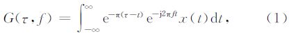
2.2 Gabor变换与S变换原理短时窗傅里叶变换的典型方法首推Gabor变换.1946年,Gabor提出了一种同时使用频率和时间来表示一个时间函数的思想和方法,这种方法便是后来的Gabor变换,连续的Gabor变换原理如公式(1)所示:
短时傅里叶变换使用一个固定的窗函数,窗函数一旦确定了以后,其形状就不再发生改变,短时傅里叶变换的分辨率也就确定了,如果要改变分辨率,则需要重新选择窗函数(廖新华等,1990;江国明等,2014).当非平稳的地震信号变化剧烈时,要求窗函数有较高的时间分辨率;而波形变化比较平缓时,则要求窗函数有较高的频率分辨率.S变换(Stockwell,1999)作为一种比较新的时频分析方法,与短时窗傅里叶变换相比,更适用于地震信号时频分析.
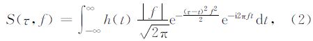
为了解决时间分辨率和频率分辨率这个矛盾,从而实现更好的时频局部化分析,Stockwell等学者于1996年引入了S变换这一数字信号处理技术.Stockwell变换的公式可以从短时窗傅里叶变换公 式出发推导得到,Stockwell等(Stockwell et al.,1996;Herman and Stockwell,2006;Letso and Stockwell,2006;Rose et al.,2006;Stockwell,2006a;Stockwell,2006b;Stockwell et al.,2006)曾经做过详细的推导,并且从理论角度论述了S变换与短时窗傅里叶变换 之间的关系.连续Stockwell变换原理如公式(2)所示:
首先,设计一组理论数据,选取反射地震中的两类典型子波函数,第一组为脉冲函数,如图 1(a,b)所示,其中1a为狄拉克δ函数,即单位脉冲函数,1b为两个单位脉冲函数的组合,代表两个脉冲事件.第二组为地震子波函数,如图 1(c,d)所示,其中图 1c为零相位子波函数,在实际反射地震资料处理中,通常通过扫描信号的互相关后获得,1d为两个振幅大小不同,极性相反的两个子波函数的组合函数.

|
图 1 实验数据 (a)脉冲函数1;(b)脉冲函数2;(c)地震子波函数1;(d)地震子波函数2. Fig. 1 Experimental data (a)Spike 1;(b)Spike 2;(c)Wavelet 1;(d)Wavelet 2. |
图 2是对图 1中的数据经过S变换得到时频谱图:其图(a)、(b)、(c)、(d)分别与图 1中(a)、(b)、(c)、(d)相互对应.变换的频谱振幅用颜色表示,其中红色表示时频谱值相对较高,蓝色表示时频谱值相对较低.图 2a中显示1 s处的脉冲信号频带覆盖很宽,并且各个频段能量相对分布均匀,这与抽象脉冲函数的频带无限宽这一事实相符合;对于图 2b所反映的两个脉冲信号,图中不仅反映了脉冲信号的频谱特征,而且准确的分辨了两个脉冲时间发生的时间,分别为0.9 s和1.1 s附近;图 2c中出现明显的频谱能量圈闭,反映图 1c中的整个信号,图中红色出现在1 s附近,代表信号能量在此处振幅相对最高,信号的频率范围为20~70 Hz之间,这与实验数据相符合;图 2d中在0.9 s和1.1 s附近分别出现能量圈闭,说明信号在这两处分别出现局部振幅或能量最大,图中可以看出,两处代表能量的颜色不同,代表信号在这两处振幅大小不同,这与图 1d所表示信号相一致.

|
图 2 实验数据S变换频谱 (a)脉冲函数1的S变换谱;(b)冲击函数2的S变换谱;(c)子波函数1的S变换谱;(d)子波函数2的S变换谱. Fig. 2 S-transform spectrum of experimental data (a)S-transform spectrum of spike 1;(b)S-transform spectrum of spike 2; (c)S-transform spectrum of wavelet 1;(d)S-transform spectrum of wavelet 2. |
需要注意的是,时频变换与傅里叶变换不同,傅里叶变换是信号在整个时域内的积分,其频谱只是信号频率的整体效应,没有局部化分析信号的功能,而S变换作为时频变换方法能够把频域和时域信息很好的结合起来,进一步分析地震资料频率随时间 的变化情况,S变换更适用于处理非平稳的地震信号.
3.2 单道数据及时频分析方法对比为了说明S变换具有的独特信号时频识别特征,本文提取典型深部低频单道数据,分别使用Gabor变换和S变换做时频谱分析,说明不同时频分析方法在识别弱信号方面的差别.具体截取深地震反射中某道第12~13 s的深部数据,如图 3a所示,分别应用Gabor变换和S变换进行对比.

|
图 3 地震道Gabor变换和S变换 (a)地震道;(b)地震道Gabor变换谱;(c)地震道S变换谱. Fig. 3 Gabor and S-transform of seismic data (a)Seismic trace;(b)Gabor transform spectrum of seismic data;(c)S-transform spectrum of seismic trace. |
从图 3a地震记录上看,地震数据波形随时间变 化明显,强的振幅分别出现在12.2 s左右,图 3(b、c)分别为地震单道的Gabor变换时频谱和S变换时频谱,对比两图,可以看到两种能够很好的刻画信号的时频特征,可以清楚地看到频率随时间的变化情况,并且从频谱图上可以明显的识别出地震异常,二者对地震数据的变换结果相对一致,同时在12.3 s、 12.6、12.8 s左右出现三处谱极值,对应主频为15~28 Hz. 然而在分辨率方面,如图 3b所示,Gabor变换在整个时间序列分辨率较低,而S变换的结果在整个时间序列对应的频段都具有良好的分辨率,可以看出S变换比Gabor变换时频谱聚焦能力更强,并且对于信号的刻画更加精细.
通过对比图 3b和3c之间可以看出,Gabor 变换在分析低频深反射地震数据时存在缺陷,这是由于Gabor 变换的时频窗口的形状一旦选定就是不可改变的,窗函数的选择决定了时间分辨率和频率分辨率,不能根据待分析信号频率的变化而改变分辨率;而在地震信号的时频分析中,要求对于低频数据信号获得较高的频率分辨率,反之对于高频信号获得较高的时间分辨率,这就要求窗函数具有随信号频率的变化而自适应的调节时窗宽度和频带宽度. 以Gabor 变换为代表的短时窗傅里叶变换无法很好的满足地震信号的时频分析要求;S变换不仅具有很好的时间分辨率,而且具有很高的频率分辨率,说明S变换具有良好的多尺度分辨能力.其本质原因是S变换可以在低频时使用较长的时窗宽度,获得较高频率分辨率,在高频时则使用较短的时窗宽度,从而得到较高的时间分辨率.S变换能精确地标定深反射地震弱信号在各个时刻的频谱,不但具有时频两域局部化分析的能力,而且能够根据不同信号的特点自动调节分辨率,其时频分析能力比Gabor变换更强,适合选作深反射地震信号的谱分解时所需的窗函数选用方法.
3.3 深地震叠加剖面及实际应用为了验证研究所用方法的有效性,使用来自地质科学院在长江中下游中段布设的深反射地震测线的反射地震数据,针对此数据进行处理,基本流程如下:首先,对输入的地震数据,选取典型道计算频谱范围,对比不同的频谱分解方法,确定谱分解方法及分解参数;其次,遍历所有地震道数据,分析频谱结果和频率道集,得到二维叠加剖面的的时频分布,根据地震信号频谱分布范围,提取对应的时频剖面.
选取数据为长江中下游地区岳西—郯庐段深地震反射资料,地震数据采用大药量爆炸源激发,CDP 范围为500~1100,采样率2 ms,截取时间范围13~15 s,如图 4所示.

|
图 4 岳西—郯庐地震叠加剖面及Gabor变换和S变换谱分解剖面 (a)地震叠加剖面;(b)Gabor变换谱分解剖面;(c)S变换谱分解剖面. Fig. 4 Yuexi-Tanlu seismic stack profile with S transform and Gabor transform spectrum decomposition profile (a)Seismic stack profile;(b)Gabor transform spectrum decomposition;(c)S transform spectrum decomposition. |
为了使深部的精细结构能较好地成像,吕庆田等在长江中下游深反射地震资料处理中,采用了针对深反射地震的剩余静校正和精细速度获取等一系列特殊成像处理(吕庆田等,2014),如图 4a所示,记录上13~13.5 s换算深度约39~40.5 km处的反射事件很难使用常规处理手段直接得到,而图中时间剖面A区中间部分所示深反射事件尤为明显,表现为反射性极强的层状密集连续反射,但B区域反射事件相对较弱,其原因一是深反射地震中来自深部的有效低频信号与深部的低频噪声频带基本重合在一起,从而在叠加剖面上,B区表现出反射同相轴连续性较弱的现象,很难直接从剖面中分辨出来;二是不同于常规石油反射,其随机噪声一般都分布在高频段,深反射地震中随机噪声还包含低频信号;三是深反射中低频和高频有效信号能量都较弱.为了更好的提取深部低频有效信号,分别采用Gabor变换和S变换两种时频谱分解方法,对不同时间、深度和对应的不同频段信号,采用不同的参数和手段处理,得到不同的时频谱分解剖面.
采用Gabor变换的时频谱分解剖面如图 4b所示,图上A、B 区域与图 4a剖面对比发现:A区域两端反射同相轴更为明显,但A区域中部同相轴连续性较4a弱,通过Gabor变换的时频谱分解剖面基本可以判断,图 4b 中A区两端反射与4a中部反射为同一反射事件.图中B区域对比发现:4a中较难直接分辨的反射事件在4b中表现为强烈的反射同相轴,从而能够明显确认B区的反射事件.综合对比图 4(a、b)中A、B区域,发现经过Gabor变换的时频谱分解剖面,深部弱反射有效信号信噪比明显提高,抑制了一部分低频噪声,同时Gabor时频谱分解也提高了深部有效信号的成像分辨率,但反射事件的同相轴连续性表现的较为破碎,这是由于在Gabor变换方法中采用了固定窗函数的效应.
S变换的时频谱分解剖面如图 4c所示,首先与图 4b对比发现:A区域层状密集连续反射区两端弱反射进一步加强,同时两侧同相轴连续性有所提高,A区中部反射事件细节刻画更加明显;其次图 4b中表现为强烈的反射同相轴的B区域,在图 4c中成像效果进一步提升,以B区整体的反射同相轴的连续性对比更为直观.
综合对比图 4(a、b、c)成像效果,深部以S变换谱分解剖面成像最优,以Gabor变换的时频谱分解剖面虽然在弱反射信号增强方面效果明显,但在事件同相轴连续性方面较以S变换谱分解剖面差,主要原因在于,以Gabor变换的时频分解方法的窗函数是定长的,窗口大小不会随着信号频率的变化来调节长度,只能在处理的过程中根据一定的记录长度范围选取窗函数参数,使得Gabor变换谱分解方法具有一定的局限性;而S变换的谱分解方法在窗函数的选取时,通过时变信号的局部频率特征自动调节窗口长度,能够更好的刻画各个频段的细节特征,在深反射剖面成像应用中效果尤为明显.
4 结论及展望本研究基于时频谱分解的方法,通过设计理论实验数据验证方法的有效性,针对深反射地震资料的单道和叠加剖面数据,对比分析了Gabor变换谱分解和S变换谱分解的应用效果,认为:
1)谱分解技术的核心在于变换窗函数的选取,基于S变换的谱分解技术是提取深反射地震资料有效低频信号的更好方法,相比短时傅里叶变换代表的Gabor变换,S变换能够精确地标定深反射地震弱信号在各个时刻的频谱,具有自动调节分辨率的能力,适合选作深反射地震信号的谱分解方法.
2)S变换谱分解技术在深地震叠加剖面上的应用有效地提高了来自深部弱反射信号的信噪比和分辨率,并刻画出了叠加剖面上所不具有的低频细节特征;S变换谱分解方法是一种比较理想的工具,适合应用于深反射弱信号的处理.
本文主要对比研究了谱分解技术在深反射地震中的应用,有待对谱分解剖面进一步剖析,结合已有的区域地质和地球物理资料,从而对测线覆盖区域的构造演化和动力学过程有更加详细深入的认识.
致谢 感谢地质科学院矿产资源研究所吕庆田研究员和审稿人对本研究的宝贵建议;部分图件采用科罗拉多矿业大学(CWP)波动现象研究中心(CSM)开源软件Seismic Unix 软件绘制,在此一并致谢.
| [1] | Askari R, Siahkoohi H R. 2008. Ground roll attenuation using the S and x-f-k transforms. Geophysical Prospecting, 56(1): 105-114. |
| [2] | Baraniuk R G, Coates M, Steeghs P. 2001. Hybrid linear/quadratic time-frequency attributes. IEEE Transactions on Signal Processing, 49(4): 760-766. |
| [3] | Bonar D, Sacchi M. 2013. Spectral decomposition with f-x-y preconditioning. Geophysical Prospecting, 61(S1): 152-165. |
| [4] | Braga I L S, Moraes F S. 2013. High-resolution gathers by inverse Q filtering in the wavelet domain. Geophysics, 78(2): V53-V61. |
| [5] | Cai H P, He Z H, Gao G, et al. 2013. Seismic data matching pursuit using hybrid optimization algorithm and its application. Journal of Central South University (Science and Technology) (in Chinese), 44(2): 687-694. |
| [6] | Chen X H, He Z H, Huang D J, et al. 2009. Low frequency shadow detection of gas reservoirs in time-frequency domain. Chinese J. Geophys. (in Chinese), 52(1): 215-221. |
| [7] | Chen X H, He Z H, Pei X G, et al. 2013a. Numerical simulation of frequency-dependent seismic response and gas reservoir delineation in turbidites: A case study from China. Journal of Applied Geophysics, 94: 22-30. |
| [8] | Chen Y P, Peng Z M, He Z H, et al. 2013b. The optimal fractional Gabor transform based on the adaptive window function and its application. Applied Geophysics, 10(3): 305-313. |
| [9] | RCoskun E, Özder S, Kocahan Ö, et al. 2007. The determination of birefringence dispersion in nematic liquid crystals by using the S-transform // Cetin S A, Hikmet I. Six International Conference of the Balkan Physical Union. Istanbul, Turkey, 899: 439-440. |
| [10] | Di C L, Yang X H, Wang X C. 2014. A four-stage hybrid model for hydrological time series forecasting. Plos One, 9(8): e104663. |
| [11] | Evans J R, Zucca J J. 1988. Active high-resolution seismic tomography of compressional wave velocity and attenuation structure at Medicine Lake Volcano, Northern California cascade range. Journal of Geophysical Research-Solid Earth, 93(B12): 15016-15036. |
| [12] | Gandhi T, Panigrahi B K, Santhosh J, et al. 2012. Contribution of brain waves for visual differences in animate and inanimate objects in human brain. Journal of Computational and Theoretical Nanoscience, 9(2): 233-242. |
| [13] | Gao J H, Chen W C, Li Y M, et al. 2003. Generalized S transform and seismic response analysis of thin interbeds. Chinese J. Geophys. (in Chinese), 46(4): 526-532. |
| [14] | Gao R, Wang H Y, Ma Y S, et al. 2006. Tectonic relationships between the Zoigê basin of the song-pan block and the west qinling orogen at lithosphere scale: results of deep seismic reflection profiling. Acta Geoscientica Sinica (in Chinese), 27(5): 411-418. |
| [15] | Han L, Sacchi M D, Han L G. 2014. Spectral decomposition and de-noising via time-frequency and space-wavenumber reassignment. Geophysical Prospecting, 62(2): 244-257. |
| [16] | Herman A G, Stockwell B R. 2006. Enzyme annotation with chemical tools. Chemistry & Biology, 13(10): 1013-1014. |
| [17] | Huang Y, Xu D, Wen X K. 2013. Optimization of wavelets in multi-wavelet decomposition and reconstruction method. Geophysical Prospecting for Petroleum (in Chinese), 52(1): 17-22. |
| [18] | Jiang G M, Zhang G B, Lü Q T, et al. 2014. Deep geodynamics of mineralization beneath the Middle-Lower Reaches of Yangtze River: Evidence from teleseismic tomography. Acta Petrologica Sinica (in Chinese), 30(4): 907-917. |
| [19] | Jiang T, Xu X C, Jia H Q, et al. 2014. Study on deep seismic reflection profile in Xingcheng area of the western Liaoning Province. Chinese J. Geophys. (in Chinese), 57(9): 2833-2845, doi: 10.6038/cjg20140910. |
| [20] | Jing J E, Wei W B, Chen H Y, et al. 2012. Magnetotelluric sounding data processing based on generalized S transformation. Chinese J. Geophys. (in Chinese), 55(12): 4015-4022, doi: 10.6038/j.issn.0001-5733.2012.12.013. |
| [21] | Leonowicz Z, Lobos T, Wozniak K. 2009. Analysis of non-stationary electric signals using the S-transform. Compel-The International Journal for Computation and Mathematics in Electrical and Electronic Engineering, 28(1): 204-210. |
| [22] | Letso R R, Stockwell B R. 2006. Chemical biology: Renewing embryonic stem cells. Nature, 444(7120): 692-693. |
| [23] | Li M, Gu X K, Shan P W. 2008. Time-frequency distribution of encountered waves using Hilbert-Huang transform. International Journal of Mechanics, 2(1): 27-32. |
| [24] | Li S J, Shi X J, Zheng H M, et al. 2002. The consistent correction of seismic amplitude in complicated surface area. Chinese J. Geophys. (in Chinese), 45(6): 862-869. |
| [25] | Li W H, Gao R, Keller Randy et al. 2014. Crustal structure of the northern margin of north China craton from Huailai to Sonid Youqi profile. Chinese J. Geophys. (in Chinese), 57(2): 472-483, doi: 10.6038/cjg20140213. |
| [26] | Liang F, Lü Q T, Yan J Y, et al. 2014. Deep structure of Ningwu volcanic basin in the Middle and Lower Reaches of Yangtze River: Insights from reflection seismic data. Acta Petrologica Sinica (in Chinese), 30(4): 941-956. |
| [27] | Liao X H, Yan P F, Chang T. 1990. Automatic faults recognition using spetrum decomposition. Acta Geophysica Sinica (in Chinese), 33(2): 220-226. |
| [28] | Lü Q T, Liu Z D, Tang J T, et al. 2014. Upper crustal structure and deformation of Lu Zong ore district: Constraints from integrated geophysical data. Acta Geologica Sinica (in Chinese), 88(4): 447-465. |
| [29] | Lu W K. 2013. An accelerated sparse time-invariant Radon transform in the mixed frequency-time domain based on iterative 2D model shrinkage. Geophysics, 78(4): V147-V155. |
| [30] | Ma Y W, Margravel G F. 2008. Seismic depth imaging with the Gabor transform. Geophysics, 73(3): S91-S97. |
| [31] | Man W S, Gao J H. 2009. Statistical denoising of signals in the S-transform domain. Computers & Geosciences, 35(6): 1079-1086. |
| [32] | Mansinha L, Stockwell R G, Lowe R P, et al. 1997. Local S-spectrum analysis of 1-D and 2-D data. Physics of the Earth and Planetary Interiors, 103(3-4): 329-336. |
| [33] | Margrave G F, Gibson P C, Grossman J P, et al. 2005. The Gabor transform, pseudodifferential operators, and seismic deconvolution. Integrated Computer Aided Engineering, 12(1): 43-55. |
| [34] | Margrave G F, Lamoureux M P, Henley D C. 2011. Gabor deconvolution: Estimating reflectivity by nonstationary deconvolution of seismic data. Geophysics, 76(3): W15-W30. |
| [35] | Mohebian R, Yari M, Riahi M A, et al. 2013. Channel detection using instantaneous spectral attributes in one of the SW Iran oil fields. Bollettino Di Geofisica Teorica Ed Applicata, 54(3): 271-282. |
| [36] | Parolai S. 2009. Denoising of seismograms using the S transform. Bulletin of the Seismological Society of America, 99(1): 226-234. |
| [37] | Pinnegar C R, Mansinha L. 2003. The S-transform with windows of arbitrary and varying shape. Geophysics, 68(1): 381-385. |
| [38] | Qi G, Lü Q T, Yan J Y, et al. 2014. 3D geological modeling of luzong ore district based on priori information constrained. Acta Geologica Sinica (in Chinese), 88(4): 466-477. |
| [39] | Reine C, van der Baan M, Clark R. 2009. The robustness of seismic attenuation measurements using fixed- and variable-window time-frequency transforms. Geophysics, 74(2): WA123-WA135. |
| [40] | Rose S, Jackson M J, Smith L A, et al. 2006. The novel adenosine A2a receptor antagonist ST1535 potentiates the effects of a threshold dose of L-DOPA in MPTP treated common marmosets. European Journal of Pharmacology, 546(1-3): 82-87. |
| [41] | Saravanan N, Siddabattuni V N S K, Ramachandran K I. 2008. A comparative study on classification of features by SVM and PSVM extracted using Morlet wavelet for fault diagnosis of spur bevel gear box. Expert Systems with Applications, 35(3): 1351-1366. |
| [42] | Sattari H, Gholami A, Siahkoohi H R. 2013. Seismic data analysis by adaptive sparse time-frequency decomposition. Geophysics, 78(5): V207-V217. |
| [43] | Song W, Zou S F, Ouyang Y L, et al. 2013. Three parameter time-frequency characteristics filter based on fast matching pursuit. Oil Geophysical Prospecting (in Chinese), 48(4): 519-525. |
| [44] | Stockwell D M. 2006a. PETR 41-FCC regenerator simulation by Lambda Sweep testing. Abstracts of Papers of the American Chemical Society, 232. |
| [45] | Stockwell D M. 2006b. PETR 73-Intra-particle mass transfer and contact time effects in FCC. Abstracts of Papers of the American Chemical Society, 232. |
| [46] | Stockwell J W Jr. 1999. The CWP/SU: Seismic Un*x package. Computers & Geosciences, 25(4): 415-419. |
| [47] | Stockwell P J, Wessell N, Reed D R, et al. 2006. A field evaluation of four larval mosquito control methods in urban catch basins. Journal of the American Mosquito Control Association, 22(4): 666-671. |
| [48] | Stockwell R G, Mansinha L, Lowe R P. 1996. Localization of the complex spectrum: The S transform. IEEE Transactions on Signal Processing, 44(4): 998-1001. |
| [49] | Suvichakorn A, Ratiney H, Bucur A, et al. 2008. Morlet wavelet analysis of magnetic resonance spectroscopic signals with macromolecular contamination.// 2008 IEEE International Workshop on Imaging Systems and Techniques. Crete: IEEE, 321-325. |
| [50] | Tang B, Yin C. 2001. Non-minimum phase seismic wavelet reconstruction based on higher order statistics. Chinese Journal of Geophysics (in Chinese), 44(3): 404-410. |
| [51] | Tao L, Gu J J, Zhuang Z Q. 2002. Two-layer parallel lattice structures of time-recursive algorithms for 2D real-valued discrete Gabor transforms.// Electronic Imaging and Multimedia Technology III. Shanghai, China: SPIE, 4925: 280-289. |
| [52] | Tary J B, Herrera R H, Han J J, et al. 2014. Spectral estimation-What is new? What is next?. Reviews of Geophysics, 52(4): 723-749. |
| [53] | Todorovska M I, Trifunac M D. 2007. Earthquake damage detection in the Imperial County Services Building-I: The data and time-frequency analysis. Soil Dynamics and Earthquake Engineering, 27(6): 564-576. |
| [54] | Xu Y Q, Sun M, Guo M S. 2007. Morlet Wavelet chaotic neural networks with random noise. Dynamics of Continuous Discrete and Impulsive Systems-Series B-Applications & Algorithms, 14: 661-666. |
| [55] | Yang W C. 1986. A generalized inversion technique for potential field data processing. Acta Geophysica Sinica (in Chinese), 29(3): 283-291. |
| [56] | Zhang Z, Yin X Y, Hao Q Y. 2014. frequency-dependent fluid identification method based on avo inversion. Chinese Journal of Geophysics (in Chinese), 57(12): 4171-4184, doi: 10.6038/cjg20141228. |
| [57] | Zhao W J, Nelson K D, Che J K, et al. 1996. Deep seismic reflection in himalaya reqion reveals the complexity of the crust and upper mantle structure. Acta Geophysica Sinica (in Chinese), 39(5): 615-628. |
| [58] | 蔡涵鹏, 贺振华, 高刚等. 2013. 基于混合优化算法的地震数据匹配追踪分解. 中南大学学报(自然科学版), 44(2): 687-694. |
| [59] | 陈学华, 贺振华, 黄德济等. 2009. 时频域油气储层低频阴影检测. 地球物理学报, 52(1): 215-221. |
| [60] | 高静怀, 陈文超, 李幼铭等. 2003. 广义S变换与薄互层地震响应分析. 地球物理学报, 46(4): 526-532. |
| [61] | 黄跃, 许多, 文雪康. 2013. 多子波分解与重构中子波的优选. 石油物探, 52(1): 17-22. |
| [62] | 高锐, 王海燕, 马永生等. 2006. 松潘地块若尔盖盆地与西秦岭造山带岩石圈尺度的构造关系—深地震反射剖面探测成果. 地球学报, 27(5): 411-418. |
| [63] | 江国明, 张贵宾, 吕庆田等. 2014. 长江中下游地区成矿深部动力学机制: 远震层析成像证据. 岩石学报, 30(4): 907-917. |
| [64] | 姜弢, 徐学纯, 贾海青等. 2014. 辽西兴城地区深反射地震剖面初步研究. 地球物理学报, 57(9): 2833-2845. |
| [65] | 景建恩, 魏文博, 陈海燕等. 2012. 基于广义S变换的大地电磁测深数据处理. 地球物理学报, 55(12): 4015-4022, doi: 10.6038/j.issn.0001-5733.2012.12.013. |
| [66] | 李生杰, 施行觉, 郑鸿明等. 2002. 复杂地表条件反射振幅一致性校正. 地球物理学报, 45(6): 862-869. |
| [67] | 李文辉, 高锐, Keller Randy等. 2014. 华北克拉通北缘(怀来—苏尼特右旗)地壳结构. 地球物理学报, 57(2): 472-483, doi: 10.6038/cjg20140213. |
| [68] | 梁锋, 吕庆田, 严加永等. 2014. 长江中下游宁芜火山岩盆地深部[CM)][LL] 结构特征——来自反射地震的认识. 岩石学报, 30(4): 941-956. |
| [69] | 廖新华, 阎平凡, 常迵. 1990. 基于谱分解的断层自动识别. 地球物理学报, 33(2): 220-226. |
| [70] | 吕庆田, 刘振东, 汤井田等. 2014. 庐枞矿集区上地壳结构与变形: 综合地球物理探测结果. 地质学报, 88(4): 447-465. |
| [71] | 祁光, 吕庆田, 严加永等. 2014. 基于先验信息约束的三维地质建模: 以庐枞矿集区为例. 地质学报, 88(4): 466-477. |
| [72] | 宋炜, 邹少峰, 欧阳永林等. 2013. 快速匹配追踪三参数时频特征滤波. 石油地球物理勘探, 48(4): 519-525. |
| [73] | 唐斌, 尹成. 2001. 基于高阶统计的非最小相位地震子波恢复. 地球物理学报, 44(3): 404-410. |
| [74] | 杨文采. 1986. 用于位场数据处理的广义反演技术. 地球物理学报, 29(3): 283-291. |
| [75] | 张震, 印兴耀, 郝前勇. 2014. 基于AVO反演的频变流体识别方法. 地球物理学报, 57(12): 4171-4184, doi: 10.6038/cjg20141228. |
| [76] | 赵文津, Nelson K D, 车敬凯等. 1996. 深反射地震揭示喜马拉雅地区地壳上地幔的复杂结构. 地球物理学报, 39(5): 615-628. |