 2015, Vol. 58


The ETAS model was fitted to the earthquake sequence of the Ludian, Yunnan MS6.5 earthquake for examining the stability of early-estimation sequence parameters and relationships among those parameters, with cutoff magnitude ML2.0, and the starting time fixed by C0=0.049 day, the ending time from 2.00 days to 149.20 days by sliding with 0.05 day steps and a total of 2945 time periods in ETAS fitting. The ETAS-based thinning algorithm was used to forecast the future next-day and 3-days aftershock rate in all the time periods, and a statistical method N-test was used to test the efficiency of such a continuous forecasting.
The parameters are μ=0.0000, K=0.0103, c=0.0039, α=1.8180 and p=0.8018 for the ETAS fitting in the Ludian, Yunnan MS6.5 earthquake sequence, and related triggering ability in generating secondary aftershocks, and the decay rate of aftershocks show no significant differences compared to other earthquake sequences in China mainland. The α value reduced from 3.5~3.8 to 1.6~2.0 in the early stage after the mainshock occurred since the ending time t2=5.05~5.10 days; the p value from 1.07 down to 0.78 within 25.00 days after the mainshock and remains steady at 0.72~0.85; and the b value increased from 0.80 to 0.95 gradually within 35.00 days after the mainshock, and remains steady at 0.93~0.97. Furthermore, the p and α values show a reverse change, the p and b value also show a reverse change within 35.00 days after the mainshock but no obvious correlation after this stage. There is no obvious correlation between the b and α values. The N-test result shows that the ETAS model-based thinning algorithm will fail to forecast the aftershock occurrence rate sometimes, for the different ending time selected and continues forecasting performed. For future 1-day forecasting, the failed forecasting is more dispersed when sliding the ending time of earthquake sequence, and the failure rate can reach to 12%. For the 3-day forecasting time window selected, the failure rate is about 6%, and failure forecasting exhibits relative concentration in the time axis, especially in the early stages after the mainshock.
It can be inferred that for optimizing the strategy of aftershock forecasting, the shorter forecasting time window should be used in the early stage after the mainshock, while a relatively longer forecasting time window can be used in the subsequent stages, such as a future 3-day forecasting time window.
强震发生后,利用余震序列早期的参数特征进行序列类型判定(Guo and Ogata,1997;蒋海昆等,2007; Enescu et al.,2009)和余震短期概率或发生率预测(Reasenberg and Jones,1989; Gerstenberger et al.,2005; Helmstetter et al.,2006; Werner et al.,2011; Zhuang,2011)等均具有重要的现实意义.目前国际上作为最接近真实描述余震序列活动,并可进行余震发生率预测的“传染型余震序列”(Epidemic Type Aftershock Sequence,简称ETAS)模型(Ogata,1988,1989,2001)得到广泛关注.在正在持续开展的“国际地震可预测性合作研究”(CSEP)计划中,ETAS模型作为重要的参赛模型,正在美国加州、日本等地区进行研究性实际预测检验(Werner et al.,2011; Zhuang,2011).
目前在对余震序列的ETAS模型参数讨论中,常对序列整体或主震后早期的阶段性的序列参数进行描述,例如Guo和Ogata(1997)、蒋海昆等(2007)和Enescu等(2009).但在主震后的早期阶段,由于地表变形、流体参与导致渗透率变化等因素可以导致序列参数快速调整(Kitagawa et al.,2002; Brenguier et al.,2008),矿物和变形构造的特性也影响断层愈合行为(Hickman et al.,1995; Ohtani et al.,2000; Ma et al.,2006),因此,余震序列参数可能出现显著变化.与此相对应,基于余震序列参数的短期余震发生率的实际效能,尤其是连续预测的效能需要系统和客观评价.
据中国地震台网测定,2014年8月3日16时30分在云南省昭通市鲁甸县(27.1°N,103.3°E)发生MS6.5地震,并造成重大人员伤亡,引起国内外广泛关注.由于此次地震震区构造复杂、周边先后发生2012年云南彝良、贵州会宁交界5.7级和5.6级地震等显著地震事件,对此次地震序列的ETAS模型参数和余震发生率的“跟踪式”研究具有重要的科学价值.针对上述的序列ETAS模型参数的时间变化特征和余震发生率连续预测效能评价两个问题,本研究将以云南鲁甸MS6.5地震为例,考察相关问题.
2 研究区和所用资料鲁甸MS6.5地震震区位于青藏高原东南缘的川滇交界东部地区,该地区由于是活动及变形的大凉山次级地块与相对稳定的华南地块之间的过渡带(徐锡伟等,2003; 闻学泽等,2013),发育着包括鲁甸—昭通断裂、五莲峰断裂在内的一系列NE向构造,以及包括包谷垴—小河断裂(李克昌等,1981)在内的次级NW向构造.由图 1给出的鲁甸MS6.5地震及周边地震分布可见,此次地震的余震空间展布复杂,在几乎以主震震中为中心的SE和SW向均有分布.震后对震区的野外地质调查结果表明,此次地震由NW向包谷垴—小河断裂发震,同时NE向构造裂缝及滑坡地质灾害明显、可能也参与主震的破裂过程(李西等,2014).地震重新定位结果(房立华等,2014)显示,余震在SE和SW向均有优势分布,展示了复杂的不对称共轭分布特征.张勇等(2015)研究结果表明,两条共轭断层先后破裂,共同参与了主震的破裂过程.考虑到上述的野外地质调查、余震重新定位和主震破裂过程反演结果,本文中根据余震的空间自然分布特征,将相对集中分布在26.95°N—27.30°N,103.10°E—103.50°E范围的事件作为余震序列进行研究.
 |
图 1 云南鲁甸MS6.5地震序列空间分布图 图中圆圈和圆点为2014-08-04—12-31期间的地震事件,虚线框为余震序列选取的空间范围,底图蓝色曲线为活动断裂带,右下角图中绿色矩形框为研究区范围示意图. Fig. 1 Seismicity distribution of the Ludian, Yunnan, MS6.5 earthquake sequence and events in the surrounding region The circles and dots show the recorded events from 2014-08-04 to 2014-12-31, dashed lines show the selected region of Ludian, Yunnan, MS6.5 earthquake sequence, the blue solid lines represent active faults. The green box in the inset (bottom-right) indicates the target region. |
为研究2014年鲁甸MS6.5地震序列,使用了中国地震台网中心“全国地震编目系统”提供的《全国统一正式编目》地震目录1).根据郭路杰等(2014)采用“震级-序号”法(见Huang,2006; 蒋长胜和吴忠良,2011;Zhuang et al.,2012)对鲁甸MS6.5地震序列的震级完整性分析结果表明,在主震发生后的0.049天,序列的完整性震级Mc=ML2.0.参照上述结果,本文选取鲁甸MS6.5主震发生的2014年8月3日至12月31日期间≥ML2.0地震序列,进行余震短期发生率连续预测和效能检验研究.根据上述时空选取结果,序列中ML2.0~2.9的地震371例、ML3.0~3.9的地震86例、ML4.0~4.9的地震9例,无5.0级以上余震.
1)全国地震编目系统,http://10.5.202.22/bianmu/index.jsp,查阅时间2015年3月22日.
3 序列整体的ETAS模型拟合情况3.1 时间序列ETAS模型对一维的余震序列随时间的衰减关系,在统计地震学的“时间点过程”(temporal point-process)研究中常使用泊松模型、应力释放模型以及修正的Omori-Ustu公式等进行研究,其中修正的Omori-Ustu公式(Omori,1894; Utsu,1961)得到了普遍使用.其表达式为:

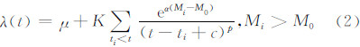
实际上真实的余震序列远比修正的Omori-Ustu公式描述的简单衰减关系复杂.为解决每个余震都可激发次级余震的情况,Ogata(1988,1989,2001)在Omori-Ustu公式基础上,提出了ETAS模型.ETAS模型假设余震遵从Omori-Ustu公式激发自己的余震,且震级的分布是独立的,在主震的发生为初始零时刻情况下,观测时间段[0,T]内的地震序列{(ti,Mi); i=1,2,…,N}的条件强度函数(conditional intensity function)可表示为(Ogata,1988):
ETAS模型的参数一般通过最大似然法(MLEs)进行估计.在地震序列目录完整的时间段[tc,T]内,0<tc < T,似然函数L的形式为:

将(2)式代入(3)式,即可对待估参数[μ,K,c,α,p]进行最大似然估计.
3.2 ETAS模型拟合情况和残差分析为考察2014年鲁甸MS6.5地震序列ETAS模型拟合的整体情况,选定序列的起始时刻C0为主震后0.049天(郭路杰等,2014),对直至2014年12月31日的Mc=ML2.0地震序列进行ETAS模型拟合.图 2a给出了利用ETAS模型拟合的鲁甸MS6.5地震序列条件强度曲线,即单位时间内的地震发生率.同时获得了ETAS模型参数,其中μ=0.0000,K=0.0103,c=0.0039,α=1.8180和p=0.8018.由图可见,在主震后38.02天震区发生ML4.3余震后,余震发生率显著增加、条件强度曲线出现明显变化.
 | 图 2 由ETAS模型拟合给出的云南鲁甸MS6.5地震序列ML2.0以上地震的条件强度曲线(a)和序列M-t图(b) Fig. 2 (a) Temporal variation of the conditional intensity from fitting the ETAS model to the Ludian, Yunnan MS6.5 earthquake sequence, with cutoff magnitude ML2.0 and (b) M-t plot |
为考察ETAS模型对鲁甸MS6.5地震序列的拟合效果,这里采用了“残差分析”方法(Ogata,1988; Daley and Vere-Jones,2003).“残差分析”方法将时间上复杂丛集的地震序列{ti}转换为齐次泊松过程,并在这种“转换时间”域{τ}进行拟合效果分析:

经过转化的数据如果与模型拟合的较好,则在{τ}上的累积频次就表现为线性,接近标准的稳态泊松过程的理论直线(Zhuang et al.,2012).图 3a给出了鲁甸MS6.5地震序列在{τ}上的累积地震数与ETAS拟合曲线比较,由图可见,在研究时段内序列的整体与ETAS模型拟合的较为理想.图 3b为与图 3a相对应的鲁甸MS6.5地震序列M-τ分布.
 |
图 3 利用ETAS模型对云南鲁甸MS6.5地震序列ML2.0以上地震的拟合情况 (a)累积地震数与ETAS拟合曲线在稳态泊松分布的“转换时间”(τ)域的比较; (b)M-τ图. Fig. 3 Comparison of the observed and modeled cumulative number of ML≥2.0 events in the Ludian, Yunnan, MS6.5 earthquake sequence (a) Observation (deep blue curve) and ETAS formula (thick dashed line) in the transformed time (τ) domain which is according to the stationary Poisson process; (b) M-τ plot. |
在利用ETAS模型进行连续、滑动的短期余震发生率预测的同时,有必要同时考察模型参数随序列持续时间的变化的稳定性.在ETAS模型参数中,α值表示激发次级余震的能力,p值表示序列的衰减特征,此外,还可单独采用最大似然法估计出相应的b值并描述余震区的应力累积状态,因此本研究中重点考察α值、p值和b值3个参数.
在云南鲁甸MS6.5地震序列ETAS模型连续、滑动拟合中,将拟合时间窗的起始时刻固定为C0=0.049天,拟合时间窗结束时刻/序列持续时间t2自主震后2.00天开始,以0.05天步长,增加至149.20天,共进行了2945个时段的时间窗滑动ETAS模型参数拟合,获得的α值、p值和b值随序列持续时间t2的变化如图 4a所示.由图可见,α值在t2=5.05~5.10天期间变化较为剧烈,由此前相对稳定的3.5~3.8急速降至此后1.6~2.0,而其后直至149.20天期间尽管也出现突增或突降现象,但变化幅度约在0.4范围内.p值在t2=2.00~25.00天期间的序列早期阶段出现趋势性的下降,自1.07逐渐下降至0.78左右,其后相对稳定地浮动在0.72~0.85之间.b值则在t2=2.00~35.00天期间逐渐增加,由0.80增至0.95,其后大致稳定在0.93~0.97之间.
 |
图 4 云南鲁甸MS6.5地震序列ETAS模型拟合参数的比较 (a)参数α值、p值和b值随序列持续时间的变化,图中分别给出了参数拟合误差;(b)参数α值和p值的分布关系;(c)参数b值和p值的分布关系;(d)参数α值和b值的分布关系.图(b)—(d)中不同颜色表示序列持续时间.序列起始时刻固定为C0=0.049天, 序列持续时间t2以0.05天步长,自主震后2.00天增加至149.20天,共进行2945个时段的滑动拟合. Fig. 4 Parameters of ETAS model in fitting the Ludian, Yunnan, MS6.5 earthquake sequence (a) The α, p and b values against the ending time (since the mainshock occurred) in ETAS fitting. The data points of α versus p values (b), b versus p values (c) and α versus b values (d) according to the figure (a). The starting time in ETAS fitting fixed by C0=0.049 day, and the ending time from 2.00 days to 149.20 days by sliding with 0.05 day steps and a total of 2945 time periods, shown in (b)—(d) by colors. |
为比较α值、p值和b值之间的时间变化特性,这里分别考察了p值与α值、p值与b值,以及b值与α值之间随t2的变化关系,分别如图 4b—4d所示.其中对于图 4b给出的p值与α值,如不考虑t2=5.10天之前α值误差较大、数值较高,以及此后t2=5.10~7.35天之间短暂的p值与α值的正比例变化外,其他时段p值与α值呈现了线性较好的反比例变化,即随着序列持续时间t2的增加,p值降低而α值增加.其次,对于图 4c给出的p值与b值,在t2<35.00天b值有趋势性升高变化的序列早期阶段,p值出现相反的减小变化,而在t2=35.00~149.20天b值稳定变化阶段,两者无明显的变化关系.上述分析表明,在主震后早期阶段随着序列衰减的减缓过程中,震源区的应力累积水平逐渐减弱(b值增加).最后,由图 4d可见,b值与α值之间无明显的规律性变化关系.
5 对余震短期发生率的连续预测和效能检验5.1 基于ETAS模型和瘦化算法的余震短期发生率预测在短期余震发生率预测研究中,通常采用Ogata(1981)发展的修正的“瘦化算法”(thinning algorithm)(Lewis and Shedler,1979)进行.“瘦化算法”基于ETAS模型的拟合参数,将地震序列转化为齐次泊松过程、外推多次模拟未来的地震发生率进行预测.其基本计算步骤如下:
(1)在进行预测/随机模拟的时段[tsta,tend]内,条件强度函数λ*的计算模型参数使用tsta时刻获得的ETAS模型参数[μ,K,c,α,p];
(2)地震序列模拟事件的发生时刻t=tsta为起点,设定序列模拟事件的“前进”时间步长函数l(t),在[t,t+l(t)]内进行齐次泊松过程模拟.其中,模拟获得的条件强度函数λ*需满足其上限低于起始时刻的条件强度函数m(t),即


(3)震级的分布函数采用

(4)如果s>l(t),设定t=t+l(t);如果t+s>tend或者U1>λ*(t+s)/m(t),则t=t+s.否则,n=n+1,tn=t+s,t=t+s;
(5)重复上述步骤,直至t+s>tend;此时生成的随机目录的时间序列为{t1,t2,…,tn}.
为连续考察云南鲁甸MS6.5地震序列的余震短期发生率预测情况,与ETAS模型参数连续拟合研究的设定规则一致,这里将拟合时间窗的起始时刻固定为C0=0.049天,序列持续时间t2自主震后2.00天开始,以0.05天步长,增加至149.20天,共进行2945个时段的连续预测.根据一般的瘦化算法应用情况,这里进行未来1天的余震发生率预测,结果如图 5所示.图 5中还同时给出了不同截止震级Mc=[2.0,3.0,…,6.0]下的预测结果.由图可见,在主震后38.02天的ML4.3等部分较强余震发生前,余震发生率预测结果有升高、概率增益增加的现象,可对强余震的预测有参考意义.
 |
图 5 利用“瘦化”算法给出的云南鲁甸MS6.5地震序列未来1天的地震发生率预测结果 图中不同颜色曲线对应不同截止震级下的地震发生率预测结果.序列起始时刻固定为C0=0.049天,序列持续 时间t2以0.05天步长,自t2=2.00天增加至t2=149.20天,共进行2945个时段的滑动预测. Fig. 5 Next-day forecasting results of the Ludian, Yunnan, MS6.5 earthquake sequence by using the thinning algorithm The curves show the forecasting results with different cut-off magnitude. The starting time in ETAS fitting fixed by C0=0.049 day, and the ending time from 2.00 days to 149.20 days by sliding with 0.05 day steps and a total of 2945 time periods. |
为定量化地检验基于ETAS模型“瘦化算法”对云南鲁甸MS6.5地震序列未来1天余震短期发生率预测的效能,这里采用了地震发生数检验的N-test方法(Kagan and Jackson,1995; Schorlemmer et al.,2007; Zechar,2010)进行考察.N-test方法基于累积泊松分布函数生成模拟地震目录,并进行不同置信度的检验.当预测的地震发生数为Nfore、模拟地震目录的累积分布函数为F时,可通过评分量δ1和δ2分别检验预测结果“至少”和“不超过”实际地震发生数Nobs的概率:
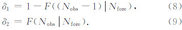
对设定的有效显著性水平αeff,当δ1<αeff表明预测的地震数目过少;当δ2<αeff时表明预测的地震数目过多.本文中设定αeff=0.025.相应的Mc=ML2.0时未来1天余震预测的N-test检验结果如图 6a所示.作为示例,图 6b—6d给出了序列持续时间t2=20.00天时的1000次模拟预测结果的统计分布,以及相应的N-test检验结果.N-test检验结果表明,对连续滑动开展的2945次预测,有58次出现δ1 < 0.025,约占总预测次数的2.0%;有285次的δ2 < 0.025,约占总预测次数的9.7%.由此表明,基于ETAS模型“瘦化算法”在对云南鲁甸MS6.5地震序列未来1天余震短期发生率预测中,约12%的情况下会出现预测失效.
 |
图 6 对云南鲁甸MS6.5地震序列未来1天地震发生率预测结果的N-test统计检验 (a)当Mc=ML2.0时不同持续时间预测结果的N-test统计检验,图中灰色垂线为δ1评分与δ2评分的连线,黑色菱形表示58次δ1 < 0.025的结果,蓝色方形表示285次δ2 < 0.025的结果;(b)序列持续时间t2=20.00天时的1000次ETAS模拟预测结果的统计分布;(c)序列持续时间t2=20.00天时的N-test检验δ1评分情况;(d)序列持续时间t2=20.00天时的N-test检验δ2评分情况. Fig. 6 N-test for the next-day forecasting results of the Ludian, Yunnan, MS6.5 earthquake sequence (a) N-test for the forecasting results with different ending time and Mc=2.0, the vertical gray dashed lines connect the δ1 and δ2 values, the black diamonds show the 58 results with δ1 < 0.025, blue squares show the 285 results with δ2 < 0.025; (b) Statistical distribution of the 1000 ETAS simulated catalogues when the ending time t2=20.00 days; (c) The δ1 score in N-test when the ending time t2=20.00 days; (d) The δ2 score in N-test when the ending time t2=20.00 days. |
由于“瘦化算法”基于ETAS模型的拟合参数进行外推预测,因此预测的时间窗的长度可能会影响预测的效能.为此,这里还针对未来3天进行预测并开展N-test检验.与1天预测时间窗的设定类似,这里仅对Mc=ML2.0的情况,将拟合时间窗的起始时刻固定为C0=0.049天,序列持续时间t2自主震后2.00天开始,以0.05天步长,增加至147.20天,共进行2905个时段的连续预测.图 7给出的结果表明,有58次出现δ1 < 0.025,占总预测次数的2.0%;有113次的δ2 < 0.025,约占总预测次数的3.9%.因此对云南鲁甸MS6.5地震序列未来3天余震短期发生率预测,约6%的情况下会出现预测失效.
 |
图 7 对云南鲁甸MS6.5地震序列未来3天地震发生率预测结果的N-test统计检验 计算中选用Mc=ML2.0,序列起始时刻固定为C0=0.049天,序列持续时间t2以0.05天步长,自主震后2.00天增加至147.20天,共进行2905次预测.图中灰色垂线为δ1评分与δ2评分的连线,黑色菱形表示58次δ1 < 0.025的结果,蓝色方形表示113次δ2 < 0.025的结果. Fig. 7 N-test for the future 3-days forecasting results of the Ludian, Yunnan, MS6.5 earthquake sequence The starting time fixed by C0=0.049 day, Mc=2.0, and the ending time from 2.00 days to 147.20 days by sliding with 0.05 day steps and a total of 2905 time periods. The vertical gray dashed lines connect the δ1 and δ2 values, the black diamonds show the 58 results with δ1 < 0.025, blue squares show the 113 results with δ2 < 0.025. |
在图 6给出的未来1天的余震发生率预测中,主震后的各个阶段均出现了预测过少和过多的情况.对比来看,图 7中未来3天的预测结果,一方面预测失效的比例由12%显著下降至6%,另一方面,预测过少的情况仅集中出现在主震后10天内的早期阶段,预测过多的情况也相对1天预测的结果在时间上更为集中.上述对比分析表明,如果采用更长的3天的预测时间窗,可相对降低预测失效的情况,但在震后的早期阶段预测过少的情况更为突出.
7 结论为研究在序列发展过程中ETAS模型参数的连续变化特征,以及基于ETAS模型的瘦化算法在余震短期发生率预测中的实际效能,本文以2014年云南鲁甸MS6.5地震序列为例,开展了ETAS模型参数连续拟合和余震短期发生率连续预测.获得了如下认识:
(1)对云南鲁甸MS6.5地震序列整体的ETAS模型拟合结果表明,参数μ=0.0000,K=0.0103,c=0.0039,α=1.8180和p=0.8018.相比较于中国大陆其他地震序列,云南鲁甸MS6.5地震序列的衰减特征、激发次级余震能力无明显差异.
(2)对云南鲁甸MS6.5地震序列ETAS模型参数的连续滑动拟合结果表明,α值在震后早期的t2=5.05~5.10天由较高的3.5~3.8急速降至1.6~2.0;p值在震后早期的t2 < 25.00天由1.07逐渐下降至0.78左右,其后稳定在0.72~0.85之间;b值则在震后早期的t2 < 35.00天逐渐由0.80增至0.95,其后稳定在0.93~0.97之间.此外,p值与α值总体呈现反比例变化; p值与b值在震后早期的t2 < 35.00天呈反比例变化,此后无明显的相关性;b值与α值之间无明显的相关性.
(3)对连续滑动预测结果的检验表明,基于ETAS模型的瘦化算法会出现部分预测失效的情况.如选用1天的预测时间窗,预测失效比例约为12%、在震后各阶段出现的较为分散;如选用3天的预测时间窗,预测失效比例为6%、在震后尤其是早期阶段集中出现.因此在余震发生率预测策略上,可在震后早期采用1天等较短的预测时间窗,而在序列参数较为稳定的后续阶段采用3天等相对较长的预测时间窗.
致谢 本文属中国地震局“云南鲁甸‘8·3’6.5级地震系统性科学考察”经费项目和“四川省芦山‘4·20’7.0级强烈地震系统性科学考察”经费项目工作.“国际地震可预测性合作研究”(CSEP)计划中国检验中心筹备组对本研究给予了指导.研究中使用了中国地震台网中心“全国地震编目系统”提供的“统一正式目录”,日本统计数理研究所庄建仓教授在访问中国地震局地球物理研究所期间编制、提供了ETAS模型和余震短期概率预测程序,并予以了指导.两位评审专家提出了诸多有益建议,对稿件的提升帮助很大,在此表示感谢.
| [1] | Brenguier F, Campillo M, Hadziioannou C, et al. 2008. Postseismic relaxation along the San Andreas fault at Parkfield from continuous seismological observations. Science, 321(5895): 1478-1481. |
| [2] | Daley D J, Vere-Jones D. 2003. An Introduction to the Theory of Point Processes-Volume 1: Elementary Theory and Methods (2nd Edition). New York, NY: Springer. |
| [3] | Enescu B, Hainzl S, Ben-Zion Y. 2009. Correlations of seismicity patterns in Southern California with surface heat flow data. Bull. Seismol. Soc. Amer., 99(6): 3114-3123. |
| [4] | Fang L H, Wu J P, Wang W L, et al. 2014. Relocation of the aftershock sequence of the MS6.5 Ludian earthquake and its seismogenic structure. Seismology and Geology (in Chinese), 36(4): 1173-1185. |
| [5] | Gerstenberger M C, Wiemer S, Jones L M, et al. 2005. Real-time forecasts of tomorrow's earthquakes in California. Nature, 435(7040): 328-331. |
| [6] | Guo L J, Jiang C S, Han L B. 2014. Parameter characteristic in the early stage of Yunnan Ludian MS6.5 earthquake sequence in 2014. Journal of Seismological Research (in Chinese), 37(4): 503-507. |
| [7] | Guo Z Q, Ogata Y. 1997. Statistical relations between the parameters of aftershocks in time, space, and magnitude. J. Geophys. Res., 102(B2): 2857-2873. |
| [8] | Helmstetter A, Kagan Y Y, Jackson D D. 2006. Comparison of short-term and time-independent earthquake forecast models for southern California. Bull. Seismol. Soc. Am., 96(1): 90-106. |
| [9] | Hickman S, Sibson R, Bruhn R. 1995. Introduction to special section: Mechanical involvement of fluids in faulting. J. Geophys. Res., 100: 12831-12840. |
| [10] | Huang Q H. 2006. Search for reliable precursors: A case study of the seismic quiescence of the 2000 western Tottori prefecture earthquake. J. Geophys. Res., 111(B4): B04301, doi: 10.1029/2005JB003982. |
| [11] | Jiang C S, Wu Z L. 2011. Intermediate-term medium-range Accelerating Moment Release (AMR) priori to the 2010 Yushu MS7.1 earthquake. Chinese J. Geophys. (in Chinese), 54(6): 1501-1510, doi: 10.3969/j.issn.0001-5733.2011.06.009. |
| [12] | Jiang H K, Zheng J C, Wu Q, et al. 2007. Earlier statistical features of ETAS model parameters and their seismological meanings. Chinese J. Geophys. (in Chinese), 50(6): 1778-1786. |
| [13] | Kagan Y Y, Jackson D D. 1995. New seismic gap hypothesis: Five years after. J. Geophys. Res., 100(B3): 3943-3959. |
| [14] | Kitagawa Y, Fujimori K, Koizumi N. 2002. Temporal change in permeability of the rock estimated from repeated water injection experiments near the Nojima fault in Awaji Island, Japan. Geophys. Res. Lett., 29(10): 121-1-121-4, doi: 10.1029/2001GL014030. |
| [15] | Lewis P A W, Shedler G S. 1979. Simulation of nonhomogeneous Poisson processes by thinning. Naval Research Logistics Quarterly, 26(3): 403-413. |
| [16] | Li K C, Hou X Y, Zhao W C, et al. 1981. The seismogeological characteristics of the Northeast Yunnan. Journal of Seismological Research (in Chinese), 4(1): 53-59. |
| [17] | Li X, Zhang J G, Xie Y Q, et al. 2014. Ludian MS6.5 earthquake surface damage and its relationship with structure. Seismology and Geology (in Chinese), 36(4): 1280-1291. |
| [18] | Ma K F, Tanaka H, Song S R, et al. 2006. Slip zone and energetics of a large earthquake from the Taiwan Chelungpu-fault Drilling Project. Nature, 444(7118): 473-476. |
| [19] | Ogata Y. 1981. On Lewis' simulation method for point processes. IEEE Transactions on Information Theory, 27(1): 23-31. |
| [20] | Ogata Y. 1988. Statistical models for earthquake occurrences and residual analysis for point processes. J. Amer. Statist. Assoc., 83(401): 9-27. |
| [21] | Ogata Y. 1989. Statistical model for standard seismicity and detection of anomalies by residual analysis. Tectonophysics, 169(1-3): 159-174. |
| [22] | Ogata Y. 1992. Detection of precursory relative quiescence before great earthquakes through a statistical model. J. Geophys. Res., 97(B13): 19845-19871. |
| [23] | Ogata Y. 2001. Increased probability of large earthquakes near aftershock regions with relative quiescence. J. Geophys. Res., 106(B5): 8729-8744. |
| [24] | Ohtani T, Fujimoto K, Ito H, et al. 2000. Fault rocks and past to recent fluid characteristics from the borehole survey of the Nojima fault ruptured in the 1995 Kobe earthquake, southwest Japan. J. Geophys. Res., 105(B7): 16161-16171. |
| [25] | Omori F. 1894. On aftershocks of earthquakes. J. Coll. Sci. Imp. Univ. Tokyo, 7: 11-200. |
| [26] | Reasenberg P A, Jones L M. 1989. Earthquake hazard after a mainshock in California. Science, 243(4895): 1173-1176. |
| [27] | Schorlemmer D, Gerstenberger M C, Wiemer S, et al. 2007. Earthquake likelihood model testing. Seismol. Res. Lett., 78(1): 17-29. |
| [28] | Utsu T. 1961. A statistical study on the occurrence of aftershocks. Geophys. Mag., 30: 521-605. |
| [29] | Wen X Z, Du F, Yi G X, et al. 2013. Earthquake potential of the Zhaotong and Lianfeng Fault zones of the eastern Sichuan-Yunnan border region. Chinese J. Geophys. (in Chinese), 56(10): 3362-3373, doi: 10.6038/cjg20131012. |
| [30] | Werner M J, Helmstetter A, Jackson D D, et al. 2011. High-resolution long-term and short-term earthquake forecasts for California. Bull. Seismol. Soc. Am., 101(4): 1630-1648. |
| [31] | Xu X W, Wen X Z, Zheng R Z, et al. 2003. Latest tectonic style and dynamic source of active blocks in Sichuan and Yunnan area. Science in China (Ser. D) (in Chinese), 33(Suppl.): 151-162. |
| [32] | Zechar J D. 2010. Evaluating earthquake predictions and earthquake forecasts: a guide for students and new researchers. Community Online Resource for Statistical Seismicity Analysis. doi: 10.5078/corssa-77337879. |
| [33] | Zhang Y, Chen Y T, Xu L S, et al. 2015. The 2014 MW6.1 Ludian, Yunnan, earthquake: A complex conjugated ruptured earthquake. Chinese J. Geophys. (in Chinese), 58(1): 153-162, doi: 10.6038/cjg20150113. |
| [34] | Zhuang J, Harte D, Werner M J, et al. 2012. Basic models of seismicity: temporal models. Community Online Resource for Statistical Seismicity Analysis. doi: 10.5078/corssa-79905851. |
| [35] | Zhuang J C. 2011. Next-day earthquake forecasts for the Japan region generated by the ETAS model. Earth Planets Space, 63(3): 207-216. |
| [36] | 房立华, 吴建平, 王未来等. 2014. 云南鲁甸MS6.5地震余震重定位及其发震构造. 地震地质, 36(4): 1173-1185. |
| [37] | 郭路杰, 蒋长胜, 韩立波. 2014. 2014年云南鲁甸6.5级地震序列参数的早期特征. 地震研究, 37(4): 503-507. |
| [38] | 蒋长胜, 吴忠良. 2011. 2010年玉树MS7.1地震前的中长期加速矩释放(AMR)问题. 地球物理学报, 54(6): 1501-1510, doi: 10.3969/j.issn.0001-5733.2011.06.009. |
| [39] | 蒋海昆, 郑建常, 吴琼等. 2007. 传染型余震序列模型震后早期参数特征及其地震学意义. 地球物理学报, 50(6): 1778-1786. |
| [40] | 李克昌, 候学英, 赵维城等. 1981. 滇东北地区地震地质特征. 地震研究, 4(1): 53-59. |
| [41] | 李西, 张建国, 谢英情等. 2014. 鲁甸MS6.5地震地表破坏及其与构造的关系. 地震地质, 36(4): 1280-1291. |
| [42] | 闻学泽, 杜方, 易桂喜等. 2013. 川滇交界东段昭通、莲峰断裂带的地震危险背景. 地球物理学报, 56(10): 3362-3373, doi: 10.6038/cjg20131012. |
| [43] | 徐锡伟, 闻学泽, 郑荣章等. 2003. 川滇地区活动块体最新构造变动样式及其动力来源. 中国科学D辑: 地球科学, 33(增刊): 151-162. |
| [44] | 张勇, 陈运泰, 许力生等. 2015. 2014年云南鲁甸Mw6.1地震: 一次共轭破裂地震. 地球物理学报, 58(1): 153-162, doi: 10.6038/cjg20150113. |