 2015, Vol. 58


2. 华北电力大学电气与电子工程学院, 北京 102206;
3. 中国电力科学研究院, 北京 100192
2. School of Electrical and Electronic Engineering, North China Electric Power University, Beijing 102206, China;
3. China Electric Power Research Institute, Beijing 100192, China
The computational results show that the abrupt changes of conductivities have influences on the induced telluric currents, which can be classified as proximity effect and skin effect. The proximity effect shows that the geoelectric field and the induced current density decrease when the conductivity varies from low to high.The minimum of geoelectric field occurs at the interface. The geoelectric fields decrease 15%, 38%, and 27% separately when the frequencies are 0.03 Hz, 0.003 Hz and 0.0005 Hz. This trend can be characterized by horizontal extent which is defined by the distance to the interface where the value becomes 1/e (=0.368) times reference value which is the difference compared to uniform structure. The horizontal extents under three frequencies are 26 km, 106 km, and 256 km. While for the case when the conductivity varies from high to low, the skin effect governs geoelectric fields at the interface by increasing 37%, 40%, and 27% at these three frequncies. The corresponding horizontal extents are 35 km, 164 km, and 283 km separately. The geoelectric field variations then increase or decrease GIC in the power systems located at the basic conductivity structure side and the mechanism is different with the impact of "coast effect". These trends and effects can be observed not only at the Earth's surface but also under the surface till the depth of 150 km. There is need to emphasize again that for GIC research in power systems, especially for those systems at coastal areas, geoelectric field and GIC should be determined taken the extension directions of transmission line and coast into consideration. Both of the proximity effect and skin effect should be considered along with coast effect in research of GIC impacts during geomagnetic disturbances.The Galerkin finite element method applied in this paper is a suitable method when modelling the more complicated conductivity structure with 3D variations. Boundary conditions discussed in this paper can be varied depending on different modelling techniques and the scales of conductivity structure models.
1 引言
磁暴时全球范围内剧烈变化的地磁场会在大地、海洋、湖泊等导电介质中感应出地电流(徐文耀,2003),并在电网、铁路网、油气管道这些与大地相连 的人工导体系统内产生地磁感应电流(geomagnetically induced currents,GIC)(Viljanen et al., 2004;刘连光等,2008).目前工程上计算GIC时,对GIC驱动源——地面电场的处理是假设其为不同方向的幅值为1 V/km的匀强电场(Overbye et al., 2013;刘连光和吴伟丽,2014),而磁暴发生时的感应电场强度可能达到几十V/km(马晓冰等,2005),并且不同地区的地面电场有显著差异(胡小静和付虹,2013;马钦忠等,2014).这种差异不仅是由于扰动地磁场变化的电流源来自于多个不同的电流体系(徐文耀等,1990;陈鸿飞和徐文耀,2001),而且易受磁暴侵害的敏感系统其空间尺度从几百公里到几千公里(Liu et al., 2014),由地球岩石圈结构的复杂性导致的电导率异常随处可见(魏文博等,2003;董树文等,2012).因此为了能够准确快速地进行地电场计算,从而正确评估GIC对敏感系统的影响,对数理模型的建模一方面要简化大范围的空间电流源和地质结构分布,另一方面要重点关注海陆岩石圈、不同板块以及板块的不同部分之间的电导率横向差异对磁暴时感应地电场和GIC的影响.
对一次场源的简化建模广泛采用的是将电流源看作位于空中一定高度的、厚度可忽略的薄片面电流或者长线电流(Pirjola,1982).对于地电导率结构的建模,目前主要采用的仍然是假定电导率只随深度变化、水平方向均匀的一维结构,包括半无限空间的均匀电导率模型(Hejda and Bochní ek,2005)或水平分层电导率模型(Liu et al., 2009;Watari et al., 2009).经过这样的简化建模以后,可以采用平面波法(Boteler,1994;Zheng et al., 2013b)、复镜像 法(Thomson and Weaver, 1975;Pirjola and Viljanen, 1998;Viljanen et al., 1999)、 FHT法(Johansen and Sørensen,1979;Hänninen et. al.,2002;Zheng et. al.,2013a)、级数展开法(Galloway et al., 1964;Pirjola et al., 1999)、SECS法(Amm and Viljanen, 1999)、复镜像与SECS相结合(Pulkkinen et al., 2003;吴伟丽和刘连光,2013)等方法求解地面感应电场的分布情况.对于广域大尺度的复杂地电结构,目前只是将整体结构分解为多个独立的一维结构,每个结构分别求解,最后将结果线性叠加(马晓冰等,2005;Viljanen et al., 2012,Marti et al., 2014).此外,由于海陆电导率的巨大差异,邻近海岸处的地电场受“海岸效应”(Boteler and Pirjola, 1998a;Boteler et al., 1998;Thomson et al., 2010;张帆等,2012)的影响要大于远离海岸的内陆地区的地电场,使得近海地区的敏感系统中更容易受到GIC的侵害和威胁.为此,Gilbert(2005)和Pirjola(2013)分别建立了海陆分界面电导率模型,在平面波为源的假设下研究了陆地侧地电场的变化情况.虽然上述方法能够快速地给出地电场分布,但针对无法推导出解析表达式的复杂地电结构建模问题,采用局部化的思路是否能准确反映电导率横向突变处电磁场的变化行为尚不确定,引入数值方法建模、探讨边界条件的施加、结合敏感系统的具体分布评估地电场的相应变化对GIC产生的影响等工作尚不多见.
为此,本文假设磁暴时扰动地磁场变化的源为位于空中一定高度的面电流,以某一水平分层地电结构为基础,构建具备各层电导率横向差异的大地电导率模型,探讨了建模计算地电场时的模型边界条件.采用伽辽金有限元法研究了不同频率的感应地电流平行于电导率横向分界面流通时,电磁场在电性突变处的分布情况,总结了电导率的横向变化影响地面电场的规律,并结合平行分界面走向的电力线路讨论了地电场变化结果对GIC的影响.
2 大地电性结构突变模式的建模与计算方法 2.1 电流源和电导率结构的建模磁暴时地面观测到的地磁场变化主要是由位于空中100 km高的电离层电流所引起(Albertson and Van Baelen,1970).假定源为位于空中100 km高、幅值为1 A/m的面电流密度.在右手直角坐标系下建立具有横向电导率突变的大地结构,规定z轴垂直向下,y轴与电导率分界面平行,x轴与分界面垂直.取z=O的平面为地平面,z>O为大地区域,z<O为空气区域,x=O处为电导率横向突变的分界面.以某个一维层状地电模型为参考(Boteler and Pirjola, 1998b),结合大地电导率分布范围(石应骏等,1985;李卫东和徐文耀,1996),建立三个电导率结构模型.模型I的电导率横向均匀,作为比较的基准;模型II和模型III的x<O区域与模型I相同,x>O区域各层厚度不变,但电导率数值分别比x<O区域大5倍和小5倍,分别模拟电导率由低导向高导突变和由高导向低导突变两种情形.只讨论源电流中与分界面平行的分量在三种结构下产生的电磁场分布情况.模型示意见图 1,地下各层的厚度和三种结构的电导率值见表 1.
 | 图 1 计算模型示意图.面电流位于地面以上100 km处,地下x<O区域的基础结构电导率保持不变,改变 x>O区域的电导率,模拟低导向高导突变、高导向低导突变的情形 Fig. 1 Sketch of computational model consisting of the sheet current 100 km above the Earth′s surface. The basic structure located at x<O is unchanged for comparison. The conductivity values at x>O are varied for modelling conductivity structures with lateral variations |
|
|
表 1 基础地电结构及横向差异地电结构数据 Table 1 Parameters of different conductivity structures |
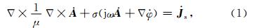
磁暴时地磁场变化的频率成份主要位于0.1~0.0001 Hz之间(Kappenman,2003;刘春明,2009),可忽略位移电流的影响.采用相量(复数)形式的矢量磁位和标量电位表述的场域控制方程为

 和
和 分别为相量(复数)形式的矢量磁位、标量电位和源电流密度,μ为空气和大地中的磁导率,磁暴计算时通常取为真空中磁导率μ0=4π×10-7H/m,σ为相应区域的电导率,ω为源变化的角频率.
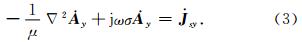
对应于图 1所示的地电结构模型,由于各场量沿y方向均匀无变化,因此可以取与xoz坐标面平 行的任意平面,将问题简化为二维场,控制方程简化为
模型的边界条件为:上下边界Γ1选取的离源区足够远,认为场在此处衰减至零,边界条件为 =0;模型的左右边界Γ2选取的离电导率突变分界面足够远,则源的几何特性决定了磁场在此处与边界垂直,边界条件为
 =0,其中的n为边界外法线方向,t为边界切线方向.地下不同电导率层的交界面条件是磁场强度的切向分量连续.
采用伽辽金有限元对式(3)进行离散化处理后得(王泽忠,2011)

面电流的变化频率选为0.03 Hz、0.003 Hz以 及0.0005 Hz(对应周期分别为30 s、300 s和1800 s),代表三种不同变化快慢的地磁扰动(Dong et al., 2013).三种频率下不同模型分界面两侧1000 km范围的地面磁场、地面电场和地面电流的幅值变化情况见图 2.由于模型I的电导率结构横向均匀,以 模型I的计算结果为基准,将其余计算结果归一化 从而更清楚地表现电导率分界面附近各量的变化情况.
 | 图 2 频率为0.03 Hz、0.003 Hz、0.0005 Hz时三种结构的归一化幅值:地面磁场(上)、地面电场(中)和 地面电流(下).实线为模型I的结果,短线为模型II的结果,点线为模型III的结果 Fig. 2 The magnitudes of geomagnetic fields(upper),geoelectric fields(middle) and telluric currents(lower)at the Earth′s surface in arbitrary units. The frequencies are 0.03 Hz,0.003 Hz, and 0.0005 Hz separately. Solid lines represent results of model I,dash lines represent results of model II and dot lines represent results of model III |
为了清晰显示各场量在地下不同区域的分布情 况,将频率为0.003 Hz时三种模型地面到地下350 km 深、分界面两侧1000 km范围内的感应地电流、地下电场和地下磁场的等值图绘于图 3.为便于结果比较,列出三种模型的地下电导率结构图.
 | 图 3 频率为0.003 Hz时三个模型地面以下350 km范围的等值图:感应地电流(上)、地下电场(中)和地下磁场(下).顶部为三种模型电导率结构图 Fig. 3 The contours of induced telluric currents(upper),electric fields(middle), and magnetic fields(lower)from the Earth′s surface to the depth of 350 km. The figures on the left are results from model I,in the middle are from model II, and on the right are from model III. The three conductivity structures are shown at the top of the contours for results comparisons. The frequency is 0.003 Hz |
对比图 2中模型I和模型II在x<O区域的结果可见,大地电导率由低导向高导突变时,靠近分界面的地面电场和地面电流会减小.地面电场的最小值出现在分界面处,频率为0.03 Hz时地面电场减小了15%;频率为0.003 Hz时减小了38%;而频率为0.0005 Hz时减小了27%.随着距分界面的距离增大,电导率横向差异的影响逐渐变得不明显.为了表征电性差异在水平方向的影响范围,以分界面处电场相对于基准值的变化幅度为单位量,定义变化幅度为单位量的1/e(=0.368)倍时,距分界面的距 离为影响宽度,用xd来表示.经计算得,频率为 0.03 Hz时,xd为26 km;频率为0.003 Hz时,xd为106 km;频率为0.0005 Hz时,xd为256 km.
对比图 2中模型I和模型III的结果可知,大地电导率由高导向低导突变时,靠近分界面的地面电场和地面电流会增大.地面电场的最大值仍位于分界面处.三种频率下分界面处的电场分别增大了37%、40%及27%.类似地,仍采用影响宽度xd来 表征结构突变的影响范围.经计算得,频率为0.03 Hz时,xd为35 km;频率为0.003 Hz时,xd为164 km;频率为0.0005 Hz时,xd为283 km.
对比图 3中模型I和模型II的结果可见,大地电性结构由低导向高导突变的过程中,会在高导一侧感生更大的地电流,影响了原结构中感应地电流的分布,使得地下各层靠近突变分界处的电流密度均减小,相应的电场和磁场也减小;而图 3中模型I和模型III的结果表明,电性结构由高导向低导突变对地下各层的影响与前者相反.这种电导率横向 突变带来的影响不仅发生在地表浅层,在地下150 km 深处仍能观察到各场量较明显的变化.
以上结果反映了电导率突变对邻近区域感应地电场的影响.具体来说,由低导向高导突变会令低导一侧的感应地电场下降,距突变分界面越远这种影响越小.对应于较高频率的地磁扰动,这种影响的范围更集中,而频率较低的地磁扰动影响的范围更广泛.而由高导向低导突变会令高导一侧的感应地电场上升,频率较高时上升的幅度较大,随着频率降低上升的幅度减小.由此可以推断,两种不同的电导率突变方式对邻近区域电场变化的影响规律并不相同.从物理本质上讲,对于同一频率的干扰源,在高导结构中会感应出幅值更大的地电流,从而改变邻近区域同方向流通的地电流分布和周围区域的场分布,这种现象称为邻近效应(冯慈璋,1979;马信山等,1995;王泽忠等,2011);而在低导结构中感应出的地电流相对较小,邻近效应表现的不明显,电导率的大幅降低使得趋肤效应成为主导因素.
由于电性结构横向突变分界面的延伸方向为y方向,各场量在该方向上不变化,若输电线路走向也为y方向,则线路上任意两接地点之间的电势差等于线路所在x处的地电场与接地点间距离的乘积.上面的计算结果表明,对低导向高导突变的情形来说,在其他条件不变的前提下,由于邻近效应的存在,线路接地点间的电势差及流通的GIC会减小,且输电线路越靠近突变分界面,减小的幅度越大.这种效应影响的水平范围与频率有关;而对于高导向低导突变的情形,相同条件下会使线路中流通的 GIC增大,且地磁变化的频率越高增大的幅度也越大.
作为与高导邻近结构类似的情形,考察线路走向与海岸线平行的输电线路中GIC的变化情况.为此,构建模型IV,假设x<O区域仍为基础结构,x>O的区域地表面到地下1 km处的电导率值为4 S/m,模拟一定深度的海水,1 km以下的区域保持基础结构不变,重点关注面电流变化频率为0.003 Hz时陆地侧各场量的变化情况,计算结果见图 4.
 | 图 4 频率为0.003 Hz时模型I与模型IV地面磁场、地面电场和地面电流的归一化幅值.实线为模型I的 结果,短线为模型IV的结果.内插图为局部放大图 Fig. 4 The magnitudes of geomagnetic fields,geoelectric fields and telluric currents at the Earth′s surface in arbitrary units. The frequency is 0.003 Hz. Solid lines represent results of model I,dash lines represent results of model IV. The inset is detail view |
对比图 4与图 2的计算结果可见,海陆结构可 看作低导向高导突变的一种极限情形.海水和陆地巨大的电导率差异使得分界面处的电场减小了66%,这将严重影响近海地区沿海岸线走向的输电线路中的GIC.而影响宽度xd为100 km,比同频率下高导邻近结构的影响宽度略小一些.
4 结论通过建立含有电导率横向突变的地电结构模型,采用伽辽金有限元法分析了磁暴期间当感应电流平行于突变分界面流通时,电导率的横向变化对地电场及地电流的影响.根据计算结果,若输电线路架设在板块交界面的一侧,另一侧为高导地质结构,会使线路所在区域的地电场减小,另一侧为低导地质结构则会使地电场增大;特别地,平行于海岸线架设的输电线路,海陆电导率差异的邻近效应会大幅减小地电场及线路中流通的GIC,这不同于“海岸效应”所描述的邻近海岸的陆地侧地电场增大、从而增大垂直海岸线架设的输电线路中的GIC.评估GIC水平需要综合考虑大地电性结构突变行为和输电线路的走向.与传统方法相比,数值方法能够准确反映电导率横向突变对地电场影响的程度和范围,并能针对复杂电导率结构进行建模和分析.
致谢 感谢芬兰气象研究院Risto Pirjola和加拿大自然资源部地磁实验室David Boteler的讨论和帮助.感谢审稿专家对本文的评阅.| [1] | Albertson V D, Van Baelen J A. 1970. Electric and magnetic fields at the Earth's surface due to auroral currents. IEEE Transactions on Power Apparatus and Systems, PAS-89(4): 578-584. |
| [2] | Amm O, Viljanen A. 1999. Ionospheric disturbance magnetic field continuation from the ground to the ionosphere using spherical elementary current systems. Earth, Planets and Space, 51(6): 431-440. |
| [3] | Boteler D H. 1994. Geomagnetically induced currents: Present knowledge and future research. IEEE Transactions on Power Delivery, 9(1): 50-58. |
| [4] | Boteler D H, Pirjola R J. 1998a. Modelling geomagnetically induced currents produced by realistic and uniform electric fields. IEEE Transactions on Power Delivery, 13(4): 1303-1308. |
| [5] | Boteler D H, Pirjola R J. 1998b. The complex-image method for calculating the magnetic and electric fields produced at the surface of the Earth by the auroral electrojet. Geophysical Journal International, 132(1): 31-40. |
| [6] | Boteler D H, Pirjola R J, Nevanlinna H. 1998. The effects of geomagnetic disturbances on electrical systems at the Earth's surface. Advances in Space Research, 22(1): 17-27. |
| [7] | Chen H F, Xu W Y. 2001. Variations of inner magnetospheric currents during the magnetic storm of May 1998. Chinese Journal of Geophysics (in Chinese), 44(4): 490-499. |
| [8] | Dong B, Danskin D W, Pirjola R J, et al. 2013. Evaluating the applicability of the finite element method for modelling of geoelectric fields. Annales Geophysicae, 31(10): 1689-1698. |
| [9] | Dong S W, Li T D, Chen X H, et al. 2012. Progress of deep exploration in mainland China: A review. Chinese J. Geophys. (in Chinese), 55(12): 3884-3901,doi:10.6038/j.issn.0001-5733.2012.12.002. |
| [10] | Feng C Z. 1979. Electromagnetic Fields (in Chinese). Beijing: People's Education Press. |
| [11] | Galloway R H, Shorrocks W B, Wedepohl L M. 1964. Calculation of electrical parameters for short and long polyphase transmission lines. Proceedings of the Institution of Electrical Engineers, 111(12): 2051-2059. |
| [12] | Gilbert J L. 2005. Modeling the effect of the ocean-land interface on induced electric fields during geomagnetic storms. Space Weather, 3(4): S04A03, doi: 10.1029/2004SW000120. |
| [13] | Hänninen J J, Pirjola R J, Lindell I V. 2002. Application of the exact image theory to studies of ground effects of space weather. Geophysical Journal International, 151(2): 534-542. |
| [14] | Hejda P, Bochníček J. 2005. Geomagnetically induced pipe-to-soil voltages in the Czech oil pipelines during October-November 2003. Annales Geophysicae, 23(9): 3089-3093. |
| [15] | Hu X J, Fu H. 2013. Analysis and research on geoelectric storm variation in Yunnan Region. Journal of Seismological Research (in Chinese), 36(4): 490-495. |
| [16] | Johansen H K, Sørensen K. 1979. Fast Hankel Transforms. Geophysical Prospecting, 27(4): 876-901. |
| [17] | Kappenman J G. 2003. Storm sudden commencement events and the associated geomagnetically induced current risks to ground-based systems at low-latitude and midlatitude locations. Space Weather, 1(3): 1016-1031. |
| [18] | Li W D, Xu W Y. 1996. Longitudinal distribution characteristics of the conductivity within the Earth's crust and upper mantle. Chinese Journal of Geophysics (in Chinese), 39(3): 322-326. |
| [19] | Liu C M. 2009. Mid-low latitude power grid geomagnetically induced currents and its assessing method[Doctor's thesis](in Chinese). Beijing: North China Electric Power University. |
| [20] | Liu C M, Liu L G, Pirjola R, et al. 2009. Calculation of geomagnetically induced currents in mid- to low-latitude power grids based on the plane wave method: A preliminary case study. Space Weather, 7(4): S04005, doi: 10.1029/2008SW000439. |
| [21] | Liu C M, Li Y L, Pirjola R. 2014. Observations and modeling of GIC in the Chinese large-scale high-voltage power networks. Journal of Space Weather and Space Climate, 4: A03. |
| [22] | Liu L G, Wu W L. 2014. Review of the influential factors of the power system disaster risk due to geomagnetic storm. Chinese J. Geophys. (in Chinese), 57(6): 1709-1719, doi: 10. 6038/cjg20140603. |
| [23] | Liu L G, Liu C M, Zhang B, et al. 2008. Strong magnetic storm's influence on China's Guangdong power grid. Chinese Journal of Geophysics (in Chinese), 51(4): 976-981. |
| [24] | Ma Q Z, Li W, Zhang J H, et al. 2014. Study on the spatial variation characteristics of the geoelectric field signals recorded at the stations in the east Huabei area when a great current is injected. Chinese J. Geophys. (in Chinese), 57(2): 518-530, doi: 10. 6038/cjg20140217. |
| [25] | Ma X B, Ferguson I J, Kong X R, et al. 2005. Effects and assessments of Geomagnetically Induced Currents (GIC). Chinese J. Geophys. (in Chinese), 48(6): 1282-1287. |
| [26] | Ma X S, Zhang J S, Wang P. 1995. Fundamentals of Electromagnetics (in Chinese). Beijing: Tsinghua University Press. |
| [27] | Marti L, Yiu C, Rezaei-Zare A, et al. 2014. Simulation of geomagnetically induced currents with piecewise layered-earth models. IEEE Transactions on Power Delivery, 29(4): 1886-1893. |
| [28] | Overbye T J, Shetye K S, Hutchins T R, et al. 2013. Power grid sensitivity analysis of geomagnetically induced currents. IEEE Transactions on Power Systems, 28(4): 4821-4828. |
| [29] | Pirjola R. 1982. Electromagnetic induction in the earth by a plane wave or by fields of line currents harmonic in time and space. Geophysica, 181(1-2): 1-161. |
| [30] | Pirjola R. 2013. Practical model applicable to investigating the coast effect on the geoelectric field in connection with studies of geomagnetically induced currents. Advances in Applied Physics, 1(1): 9-28. |
| [31] | Pirjola R, Viljanen A. 1998. Complex image method for calculating electric and magnetic fields produced by an auroral electrojet of a finite length. Annales Geophysicae, 16(11): 1434-1444. |
| [32] | Pirjola R, Viljanen A, Boteler D. 1999. Series expansions for the electric and magnetic fields produced by a line or sheet current source above a layered Earth. Radio Science, 34(2): 269-280. |
| [33] | Pulkkinen A, Amm O, Viljanen A. 2003. Ionospheric equivalent current distributions determined with the method of spherical elementary current systems. Journal of Geophysical Research: Space Physics (1978—2012), 108(A2): 1053, doi: 10.1029/2001JA005085. |
| [34] | Shi Y J, Liu G D, Wu G Y, et al. 1985. Magnetotelluric Sounding Tutorial (in Chinese). Beijing: Earthquake Press. |
| [35] | Thomson D J, Weaver J T. 1975. The complex image approximation for induction in a multilayered Earth. Journal of Geophysical Research, 80(1): 123-129. |
| [36] | Thomson A W P, Gaunt C T, Cilliers P, et al. 2010. Present day challenges in understanding the geomagnetic hazard to national power grids. Advances in Space Research, 45(9): 1182-1190. |
| [37] | Viljanen A, Amm O, Pirjola R. 1999. Modeling geomagnetically induced currents during different ionospheric situations. Journal of Geophysical Research, 104(A12): 28059-28071. |
| [38] | Viljanen A, Pulkkinen A, Amm O, et al. 2004. Fast computation of the geoelectric field using the method of elementary current systems and planar Earth models. Annales Geophysicae, 22(1): 101-113. |
| [39] | Viljanen A, Pirjola R, Magnus W, et al. 2012. Continental scale modelling of geomagnetically induced currents. Journal of Space Weather and Space Climate, 2: A17. |
| [40] | Wang Z Z. 2011. Concise Computational Electromagnetic Fields (in Chinese). Beijing: China Machine Press. |
| [41] | Wang Z Z, Quan Y S, Lu B X. 2011. Engineering Electromagnetic Fields (in Chinese). Beijing: Tsinghua University Press. |
| [42] | Watari S, Kunitake M, Kitamura K, et al. 2009. Measurements of geomagnetically induced current in a power grid in Hokkaido, Japan. Space Weather, 7(3): S03002, doi: 10.1029/2008SW000417. |
| [43] | Wei W B, Jin S, Ye G F, et al. 2003. Methods to study electrical conductivity of continental lithosphere. Earth Science Frontiers (in Chinese), 10(1): 15-22. |
| [44] | Wu W L, Liu L G, 2013. Calculation method for geoelectric field in mid- and low-latitude area based on sparse geomagnetic data. Chinese J. Space Sci. (in Chinese), 33(6): 617-623. |
| [45] | Xu W Y. 2003. Geomagnetism (in Chinese). Beijing: Seismological Press. |
| [46] | Xu W Y, Zhang M L, Lin Y F, et al. 1990. Analysis on structure of the variable geomagnetic fields at middle and low latitudes. Chinese Journal of Geophysics (in Chinese), 33(1): 12-21. |
| [47] | Zhang F, Wei W B, Jin S, et al. 2012. Ocean coast effect on land-side magnetotelluric data in the vicinity of the coast. Chinese J. Geophys. (in Chinese), 55(12): 4023-4035, doi: 10.6038/j.issn.0001-5733.2012.12.014. |
| [48] | Zheng K, Pirjola R J, Boteler D H, et al. 2013a. Geoelectric fields due to small-scale and large-scale source currents. IEEE Transactions on Power Delivery, 28(1): 442-449. |
| [49] | Zheng K, Trichtchenko L, Pirjola R J, et al. 2013b. Effects of geophysical parameters on GIC illustrated by benchmark network modeling. IEEE Transactions on Power Delivery, 28(2): 1183-1191. |
| [50] | 陈鸿飞, 徐文耀. 2001. 1998年5月磁暴磁层电流体系的地磁效应分析. 地球物理学报, 44(4): 490-499. |
| [51] | 董树文, 李廷栋, 陈宣华等. 2012. 我国深部探测技术与实验研究进展综述. 地球物理学报, 55(12): 3884-3901, doi:10.6038/j.issn.00015733.2012.12.002. |
| [52] | 冯慈璋. 1979. 电磁场. 北京: 人民教育出版社. |
| [53] | 胡小静, 付虹. 2013. 云南地区地电暴变化分析研究. 地震研究, 36(4): 490-495. |
| [54] | 李卫东, 徐文耀. 1996. 全球地壳、上地幔电导率经向分布特征. 地球物理学报, 39(3): 322-326. |
| [55] | 刘春明. 2009. 中低纬电网地磁感应电流及其评估方法研究[博士论文]. 北京: 华北电力大学. |
| [56] | 刘连光, 吴伟丽. 2014.电网磁暴灾害风险影响因素研究综述. 地球物理学报, 57(6): 1709-1719, doi: 10.6038/cjg20140603. |
| [57] | 刘连光, 刘春明, 张冰等. 2008. 中国广东电网的几次强磁暴影响事件. 地球物理学报, 51(4): 976-981. |
| [58] | 马钦忠, 李伟, 张继红等. 2014. 与大电流信号有关的华北东部地区地电场空间变化特征的研究. 地球物理学报, 57(2): 518-530, doi: 10.6038/cjg20140217. |
| [59] | 马晓冰, Ferguson I J, 孔祥儒等. 2005. 地磁感应电流(GIC)的作用与评估. 地球物理学报, 48(6): 1282-1287. |
| [60] | 马信山, 张济世, 王平. 1995. 电磁场基础. 北京: 清华大学出版社. |
| [61] | 石应骏, 刘国栋, 吴广耀等. 1985. 大地电磁测深法教程. 北京: 地震出版社. |
| [62] | 王泽忠. 2011. 简明电磁场数值计算. 北京: 机械工业出版社. |
| [63] | 王泽忠, 全玉生, 卢斌先. 2011. 工程电磁场. 北京: 清华大学出版社. |
| [64] | 魏文博, 金胜, 叶高峰等. 2003. 大陆岩石圈导电性的研究方法. 地学前缘, 10(1): 15-22. |
| [65] | 吴伟丽, 刘连光. 2013. 基于稀疏地磁数据的中低纬度磁暴感应地电场的算法研究. 空间科学学报, 33(6): 617-623. |
| [66] | 徐文耀. 2003. 地磁学. 北京: 地震出版社. |
| [67] | 徐文耀, 张满莲, 林云芳等. 1990. 中低纬度区变化地磁场的结构分析. 地球物理学报, 33(1): 12-21. |
| [68] | 张帆, 魏文博, 金胜等. 2012. 海岸效应对近海地区大地电磁测深数据畸变作用研究. 地球物理学报, 55(12): 4023-4035, doi: 10.6038/j. issn. 0001-5733.2012.12.014. |