 2015, Vol. 58


2. 中国科学院地质与地球物理研究所, 北京 100029
2. Institute of Geology and Geophysics, Chinese Academy of Sciences, Beijing 100029, China
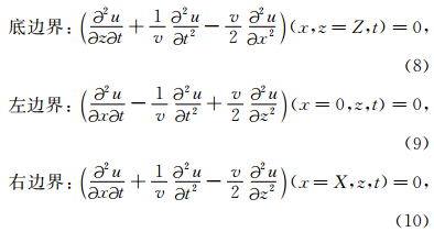
Mathematically, the prestack data can be obtained by the forward modeling of wave equations. The seismic waves generated by a Ricker wavelet source propagate through the underground media. When the waves encounter the interfaces or inhomogeneous objects with different physical parameters, they are reflected back to the surface. These reflected waves are received by the geophones on the surface and used for inversion or other seismic data processing. This process is usually modeled by wave equations such as the acoustic wave equation if we assume the underground media is acoustic. In this paper, we investigate the full-waveform velocity inversion based on the 2-D acoustic wave equation and the corresponding computations are completed in the time domain. The forward problem is to solve the acoustic wave equation numerically and obtain the prestack data. Many numerical methods can be used to solve the forward problem, for example, the finite element method and the finite volume method and so on. In this paper we adopt the finite difference method because of easy programming and its high efficiency. Since the computational domain is a bounded rectangular domain and boundary reflections may devastate inversion results, it is necessary to use the absorbing boundary conditions and eliminate boundary reflections. The boundary conditions we adopted are the second-order Clayton's absorbing boundary conditions. The computational discrete schemes for the equation and boundary conditions are of second-order accuracy both in time and space.
The inversion is required to solve a nonlinear least-square problem. It is an iterative minimization process between the synthetic data and the observed data. Aiming at the difficulty which the waveform inversion is easy to fall into local extreme points, we propose the "stepwise inversion" strategy. First we use the wavefield on the lower frequency scale to obtain a reasonable initial model. Then we use the wavefield on the other high frequency scales to do inversion step by step. In order to use the wavefield information fully, the information at large scale contain that at low scale. Moreover, the inversion result at the previous low-frequency scale is chosen as the initial model for the next inversion at the large-frequency scale. The optimization method in inversion is the L-BFGS method. The full-waveform inversion is a typical large-scale scientific computational problem and the computations are implemented based on the MPI parallel algorithm on the PC cluster.
The theoretical formulae and algorithms, including the finite-difference forward modeling, velocity model correction, gradient computation and corresponding algorithm, are expounded and derived in detail. In numerical computations, the full-waveform inversion based on the MPI parallel computations for the Marmousi model are completed. The Marmousi model is a complicated benchmark 2-D model which is usually used for testing the ability of migration and inversion methods. In the process of "stepwise inversion", the data at five different scales, i.e. 0~5 Hz, 0~10 Hz, 0~25 Hz, 0~35 Hz, 0~60 Hz, are selected. The initial model at first scale is a linear velocity model which is reasonable in practical case. The iteration inversion results at the first scale (i.e. 0~5 Hz) show that the inversion gets better as the iteration number increases till some iteration number such as the 50th iteration. This phenomenon can be observed by the variations of object function. Then we stop the inversion and the corresponding inversion result is used for the initial velocity model for the inversion at the second cale ( i.e. 0~10 Hz). The following procedure is similar till the inversion at the fifth scale (i.e. 0~60 Hz) is completed. At each scale, the inversion iteration number may be set 50 as more inversion iterations can not decline the value of object function. For comparisons, the inversion result without using the stepwise strategy is also given and shows that the iteration inversion converges to a wrong local extreme result. The detail comparisons between numerical and exact results at a fixed CDP are presented. The computations are completed on the PC cluster. The parallel efficiency is high and the scalability is about 0.9.
The full waveform inversion is an iterative process of residual minimization between synthetic data and the known records. The inversion is easy to fall into local minimum points. We develop the sequential inversion method based on the inversion with the data at different frequency scales. The main idea is that the inversion result at low frequency scale is chosen as the initial guessing model for the inversion at the next high frequency scale. This strategy effectively solves the problem of inversion divergence when the initial value is far from the true solution. The detailed descriptions including theoretical formula and the corresponding algorithms are given or derived in this paper. Numerical computations for the complex structure model named Marmousi model are carried out. Relative good inversion results are yielded. Many computations show that the method is effective and has high robustness to the initial model. The full-waveform inversion based on wave equations is a typical large scale scientific computational problem. The implementation based on the MPI algorithm improves the computational efficiency greatly, which provides the basis for further application to real data.
地震全波形反演是利用地表或钻孔中观测到的叠前波场记录信息,推测地球内部介质的物性参数,以确定含油气构造.速度是重要的物性参数之一,速度反演或建模是地球物理偏移成像和地震资料解释的重要基础.走时反演或成析成像(例如,Fawcett et al., 1985; Dahlen et al., 2000; Hung et al., 2004;Gautier et al., 2008; Tong et al., 2011)是速度反演的一种重要方法,但该方法只利用了波场的到时信息,本质上是一种高频近似方法,适于对区域背景速度场成像,对复杂速度构造模型成像精度不足.全波形反演(例如,Tarantola,1984; Mora,1987; Yang,1993; Pratt et al., 1998)利用波场的走时、振幅和相位信息来反演,具有更好的精度和更高的分辨率,但计算量大,难度大,特别是二维和三维情形.从20世纪80年代以来,人们一直致力于这方面的研究,发展了多种地震全波形反演方法,这些方法相互交叉或综合,并无严格界限,大致可如下分类.基于求解波动方程计算域的不同,可分时间域反演(例如,Tarantola,1984; Bleistein,1987; Zhang et al., 2013)、频率域反演(Pratt et al., 1988; Song,1995; Pratt et al., 1998; Pratt,1999; Sirgue et al., 2004)和Laplace域反演(Shin et al., 2008,2009; Ha et al., 2012).基于求解方 式的不同,有局部线性化梯度类迭代反演(Tarantola, 1984,1986; Gauthier et al., 1986; Bleistein,1987; Mora,1987)、混沌反演(Yang,1993)和全局搜索优化反演等.
线性反演不能恢复速度模型的长波场分量(Devancy,1984),波动方程反问题的主要方 法是非线性优化迭代反演方法和Born反演(Bleistein,1987). Tarantola首先(Tarantola, 1984,1986)对完全非线性全波形反演进行了详细的研究,数学上归结为一个局部最优化问题.求解这类问题时,扰动模型沿目标函数的梯度搜索,其中梯度可由震源激发的入射波场和残差反传播后的波场计算得到,这种方法可以避免直接通过模型参数扰动来计算Frechet导数,大大减少了计算量,使得二维时间域波动方程全波形反演成为可能,该思想已用到声波和弹性波方程的全波形反演中(Gauthier et al., 1986; Mora,1987);此外,Sheen等(Sheen et al., 2006)对弹性介质在时间域用高斯牛顿法进行了全波形反演,Choi等(Choi et al., 2008)对声学弹性复合介质中的多分量数据用共轭梯度法进行了二维全波形反演,Epanomeritakis等(Epanomeritakis et al., 2008)结合高斯牛顿法和共轭梯度法对三维弹性波方程进行了全波形反演.将时间域的声波方程和弹性波方程变换到频率域,然后对给定的频率再进行正演模拟,反演也在频率域中求解(Pratt et al., 1988; Song,1995; Pratt et al., 1998; Pratt,1999; Sirgue et al., 2004),这就是频率域全波形反演.Pratt等(Pratt et al., 1988)首先将全波形反演思想用于频率域中,频率域反演和时间域反演的思想是完全一致的,只是频率域的波场是互相解耦的,可以对每个频率单独进行反演,频率域反演对初始模型也存在较大的依赖性.类似地,全波形反演还可 在Laplace域中进行(Shin et al., 2008; Shin et al., 2009; Ha,2012).
全波形反演数值上常用迭代法来求解,总体上是一个梯度类的优化迭代求解过程,有精度高的优点,但对初始模型有严重依赖性,这是梯度类反演方法的共性.Gauthier等(1986)曾证明当初始速度模型与真实模型有10%的误差时,全波形反演就失效.在这种情况下,梯度类方法趋向找到局部极值点.为了提高全波形反演对初值的稳健性,Bunks等(1995)提出了多尺度全波形反演方法,通过将问题分解为不同尺度求解以保证反演过程稳定收敛.此外,人们还研究了用全局优化搜索的方法来求解.全局优化搜索基于随机过程,不需目标函数的导数信息,也不考虑目标函数的形状,不需要一个好的初值模型,而且不会陷入局部极值点,例如,Jin等(1994)提出了蒙特 卡洛法反演,Smabridge等(1992)提出了遗传算法反演,Sen和Stoffa(Stoffa et al., 1991; Sen et al., 1995)提出了模拟退火法.全局优化搜索由于为求得目标函数的全局极值所导致的计算量极大,特别是二维和三维反演.
依据线性化反演理论,当一个初始模型在观测数据和模拟数据之间引起大的动力学残差时,速度模型的扰动对残差的平方就没有影响,从而数据对模型参数的梯度为零,但这时求得的极值点显然不是全局极值点,这就造成速度反演的大量极值点,不但难以求得好的收敛结果或甚至发散,而且反复迭代计算也导致巨大的计算量.为此,本文研究了时间域频率多尺度全波形反演方法,提出了基于不同尺度的频率数据的逐级反演策略,取得了明显效果.
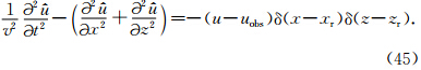
2 理论方法 2.1 有限差分正演模拟在时间域上,考虑二维声波方程:

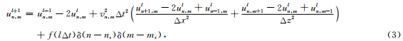
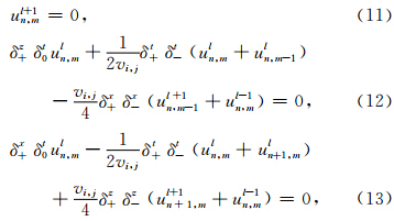
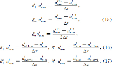
有限差分法是数值模拟波场传播的重要方法之一,具有计算效率高的优点.本文用有限差分法来求解波动方程.设Δx和Δz分别为x和z方向的离散步长,Δt为时间步长,用n,mul表示lΔt时刻及空间位置为(nΔx,mΔz)处的波场值,vn,m表示空间位置(nΔx,mΔz)处的速度离散值.用二阶中心差分格式对方程(1)进行离散,得

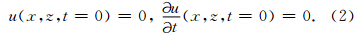
顶边界:u(x,z=0,t)=0,(7)

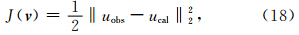
全波形反演是一个迭代极小化观测数据与拟合数据之间的残量即目标函数来反演速度v的过程.残量使用l2范数来度量,目标函数可写成:


步骤1:给定初始模型v0,迭代中止精度ε,最大迭代次数kmax,令迭代步k=0;
步骤2:对v0,计算目标函数值J和梯度g;设定初始搜索方向p0=-g;令α0=1/‖p‖2;
步骤 3:如果k
1:用一维线搜索算法,得到搜索步长αk;
2:速度模型修正vk+1=vk+αkpk;
3:对修正的vk+1,计算新的目标函数值J和梯度g:
4:若梯度或目标函数值满足终止条件,则算法终止,否则转步骤4;
5:计算新的搜索方向pk;
6:令k=k+1,返回步骤3继续.
步骤4:输出结果v.
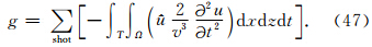
在该算法中,需要计算目标函数的梯度g,对大规模模型的计算,我们基于下面的共轭方法来计算.
2.3 梯度计算在BFGS方法中需要梯度的信息,这是一个M×(Nt×Nr)矩阵,这里Nr为接收点数.若用差分法求梯度需要求解M次的正问题,计算量太大.差分法计算梯度适合求解规模较小的问题(Zhang et al., 2013).共轭法即求解原问题的共轭问题,是大规模问题中最常用的梯度计算方法,它只需要两次正问题的计算量就可以得到一个较为准确的梯度.下面给出这种方法的一般形式的推导.记

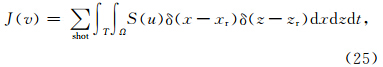

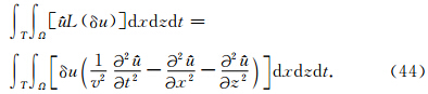
 vuδv,vu是u关于v的导数.因为u是关于v的非线性函数,vu不易直接求出,下面给出的方法是为了计算梯度时避免求解δu.为此,将正演问题写作

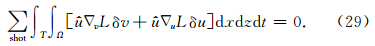
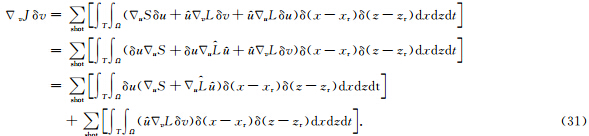
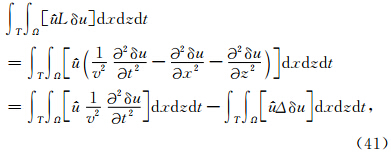
 乘以上式且对时间和空间积分,得
 使得
使得


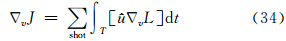
,则梯度可以由

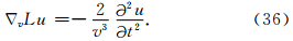
下面考虑如何求的值.假设由于速度扰动δv引起的散射场的扰动为


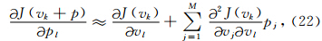
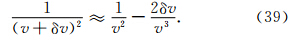
采用下列近似:
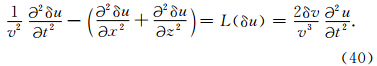
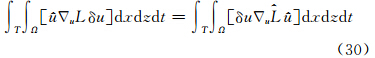
,考虑到式(30),计算
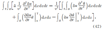
 =0,则第2项为0.等号右端第3项中,已知|t=T=0,且可令
 |t=T=0,则第3项为0. 考虑式(41)最后一个等号右端第2项,由Green公式可知:

使得边界项为0. 要求上边界为零边界条件,其他三边使用吸收边界条件,显然零边界条件使得边界项为0,对于吸收边界条件,只要吸收得比较彻底,其实可以 认为区域是无界的,这样就不需要考虑边界项的 影响,可以看出好的吸收边界对于梯度的计算是很重要的,吸收不完全会对梯度计算的准确性带来影响.
综合式(41)、(42)和(43),可以得到:
可描述为:

本节用Marmousi复杂构造模型来进行反演数值计算.图 1是Marmousi速度模型,常用来做偏移成像,用于验证各种成像方法的能力和效果(张文生,2009).数值算例实验设计如下:计算的实际规模是地表宽度2952 m,地下深度为1488 m,记录时间为1.8 s.空间步长Δx=6 m,Δz=6 m,由稳定性条件取Δt=0.6 ms. 震源的最大频率为60 Hz,中心频率为30 Hz.离散后区域的空间点数为Nx=493和Nz=249,时间取样点数为Nt=3001.实验中共设80个炮点,每个炮点有40个接收点,双边接收.接收点之间的距离均为24 m,炮检距离为24 m.炮点和接收点置放在同一水平线上,深度为6 m.
 | 图 1 Marmousi速度结构模型Fig. 1 Marmousi velocity structure model |
观测数据是由Marmousi模型正演得到的人工数据.图 2是某炮的炮记录,图 2a无边界吸收,图 2b有边界吸收,比较可以看到,边界反射得到了明显的消除,这有助于提高梯度计算的精度.图 3是用 于反演的初始速度模型图,速度范围是1500 m·s-1 至4300 m·s-1,中间每层线性递增得到的,每层速度相同;可以看到初始模型与真实模型的差异很大,已经完全没有原来真实模型的构造信息了.
 | 图 2 某炮的炮记录 (a)无边界吸收;(b)有边界吸收.Fig. 2 A shot gather record with(a)no boundar absorption, and (b)boundary absorption |
 | 图 3 初始速度模型Fig. 3 Initial velocity model |
频率多尺度方法就是根据问题对不同尺度的频率进行分解.为简单起见,我们采用截去某个频率以上的所有频率,只保留这个频率以下的频率进行反演,然后增加频率上界,依次进行反演.在本文计算中,选取的频率多尺度实验分为5个尺度:0~5 Hz,0~10 Hz,0~25 Hz,0~35 Hz,0~60 Hz;每个尺度有逐级包含关系,这样可以更有效地恢复模型波数.为作为比较,在不采用本文频率多尺度方法的情况下也直接对原始数据反演,图 4是迭代250步的结果,可以看到结果较差,再继续迭代也是如此.下面我们对5个频率尺度的波场进行逐级反演,每个尺度分别迭代50次.首先用0~5 Hz频率尺度波场进行反演,图 5a、5b和5c 分别是迭代5步、 20步和50步的反演结果,初始模型仍为图 3.可以明显看到,反演结果随迭代次数增加逐步向好的方向收敛.为了节省篇幅,下面直接给出其他尺度迭代50次的反演结果.图 6用是0~10 Hz频率尺度的波场反演迭代50次的结果,初始模型是图 5c;图 7是用0~25 Hz数据反演迭代50次的结果,初始模型是图 6;图 8是用0~35 Hz数据反演迭代50次的结果,初始模型是图 7;图 9是用0~60 Hz数据反演迭代50次的结果,初始模型是图 7.可以看到,反演 结果从图 6到图 9逐步变好;图 8和图 9的结果比较接近,不过比较可以看出在细节上还是有些差别(比较下面的图 10e和图 10f更清楚).为了进一步与真实模型作细致的比较,我们取CDP号为180处的位置,来与真实模型作比较;图 10是5个不同频率尺度迭代50次的全波形反演结果(红线)与真实模型(蓝线)的比较.比较可知,在模型浅部,有非常好的收敛,在深部,反演的精度虽不如浅部,但仍能反映出良好的构造信息.原因有两方面,一是深部波场信息相对与浅层较弱,在计算中我们未对波场作任何处理;二是从数值计算的角度看,目标函数的未知量是一个向量,分量是每个网格点的速度值,目标函数梯度的分量对应每个网格点的梯度,从而也表示了不同深度的梯度,负梯度方向是未知量的修正方向,由于浅部接收信号强,浅部的变化量即梯度就会比较大,修正的时候着重于修正浅部.目标函数的二阶导数反映每个分量变化对梯度的影响,对深浅有平衡作用,但二阶导数是近似计算的,因此不可避免会导致深部反演结果的误差大于浅部.图 11给出了0~50 Hz频率尺度反演的目标函数值随迭代步的变化情况,可以看到前30次迭代,目标函数值下降很快,在80次之后,下降很小,表明继续迭代反演结果改善也不大,其他尺度的情况大致类似,考虑到计算量,每级反演设置最大迭代次数为50.此外,我们还对加噪声的情况也进行了数值计算,结果表明对20%的随机噪声也有校好的反演结果,为节省篇幅,不再详述.
 | 图 4 不用频率多尺度方法,用0~60 Hz的波场数据迭代250次的反演结果(初始模型为图 3)Fig. 4 The inversion result after 250 iterations with 0~60 Hz wavefield data. The frequency multiscale method is not adopted(The initial model is Fig. 3) |
 | 图 5 0~5 Hz的波场数据的全波形反演结果(初始模型为图 3) (a)迭代5次;(b)迭代20次;(c)迭代50次.Fig. 5 The full-waveform inversion results with 0~5 Hz wavefield data(The initial model is Fig. 3) (a)5 iterations;(b)20 iterations;(c)50 iterations. |
 | 图 6 0~10 Hz的波场数据迭代50次的全波形反演结果(初始模型为图 5c)Fig. 6 The full-waveform inversion result with 0~10 Hz wavefield data after 50 iterations(The initial model is Fig. 5c) |
 | 图 7 0~25 Hz的波场数据迭代50次的全波形反演结果(初始模型为图 6)Fig. 7 The full-waveform inversion result with 0~25 Hz wavefield data after 50 iterations(The initial model is Fig. 6) |
 | 图 8 0~35 Hz的波场数据迭代50次的全波形反演结果(初始模型为图 7)Fig. 8 The full-waveform inversion result with 0~35 Hz wavefield data after 50 iterations(The initial model is Fig. 7) |
 | 图 9 0~60 Hz的波场数据迭代50次的全波形反演结果(初始模型为图 8)Fig. 9 The full-waveform inversion result with 0~60 Hz wavefield data after 50 iterations(The initial model is Fig. 8) |
 | 图 10 在CDP180位置处,不同频率尺度波场迭代50次的全波形反演结果(红线)与真实模型(蓝线)的比较 (a)初始模型;(b)0~5 Hz;(c)0~10 Hz;(d)0~25 Hz;(e)0~35 Hz;(f)0~60 Hz.Fig. 10 A comparison between the full-waveform inversion results after 50 iterations on five different frequency scales(red line) and the exact model(blue line)at the position of CDP 180 (a)Initial model;(b)0~5 Hz;(c)0~10 Hz;(d)0~25 Hz;(e)0~35 Hz;(f)0~60 Hz. |
 | 图 11 0~50 Hz频率多尺度反演目标函数随迭代步k的变化情况Fig. 11 The variation of objective function vale of 0~50 Hz frequency multiscale inversion with the iterative number k |
最后指出,全波形反演是一个典型的大规模科学计算问题,计算量巨大,我们采用了MPI并行算法来实现.在计算中,对计算区域进行划分,分别赋予不同进程计算,这样,问题就分布存储在各个进程中,从而满足大规模计算对内存的要求.正问题是整个区域上关于时间递推的计算,每个离散点的 计算都有它附近点进行参与,所以在进程管理区域 边界与相邻的进程之间有信息交换.显然,边界点数与子区域点数比值越小,通信时间与计算时间的比值就越小计算效率就越高.通信过多会导致并行效率变差.由BFGS算法可知,搜索方向的计算只有向量参与,没有矩阵,向量点积只需在各进程中进行计算,再将所有进程所求的值进行相加即可,注意重叠区域不要进行多次运算.下面分析一下并行效率.我们知道,串行程序的执行时间近似等于程序指令执行花费的CPU 时间,但并行程序相对复杂,其执行 时间等于从并行程序开始执行,到所有进程执行完 毕,墙上时钟走过的时间,也称之为墙上时间(Walltime).对各个进程,墙上时间包括计算CPU 时间、通信CPU 时间、同步开销时间、同步导致的进程空闲时间.表 1列出了4进程、8进程、16进程、32进程迭代反演10次的墙上计算时间的比较,由此可算出并行可扩展性.可以看到,平均的并行可扩展性大于0.9,是比较高的.计算在“科学与工程计算国家重点实验室”三号机群系统上完成,该机群有282个计算刀片,每个刀片包含两颗Intel X5550四 核处理和24 GB内存,单核双精度浮点峰值性能为10.68Gflops.用32个进程进行计算,总迭代250步,计算时间约47 h.
| 表 1 并行算法效率分析Table 1 Analysis of the efficiency of parallel algorithm |
全波形反演是一个极小化模拟数据与已知记录之间残差的迭代过程.反演在时间域中进行,针对反演易陷入局部极小值的问题,我们发展了基于不同 尺度频率数据的逐级反演方法,即用前一尺度的反 演结果作为下一尺度反演的初值模型,有效地解决了初值离真解较远时,反演不收敛的问题.文中详细阐述和推导了理论公式和相应的算法,并基于Marmousi复杂构造模型进行了大规模反演计算,得到了较好的反演结果,说明了该方法的有效性和对初始模型具有较高的稳健性.波动方程全波形反演是一个典型的大规模科学计算问题,计算量巨大,文中用MPI并行方法来实现,提高了计算效率,这为进一步应用提供了基础.
致谢 本文的计算在科学与工程计算国家重点实验室三号机群系统上完成,在此表示感谢,此外还要感谢实验室很多老师的大力帮助和支持,在此不一一指出.最后,还要感谢审稿者提出的宝贵建议,使得本文能以目前的形式呈现.| [3] | Berenger J P. 1994. A perfectly matched layer for the absorption of electromagnetic waves. J. Comput. Phys., 114(2): 185-200. |
| [4] | Bleistein N, Cohen J K, Hagin F G. 1987. Two and one-half dimensional Born inversion with an arbitrary reference. Geophysics, 52(1): 26-36. |
| [5] | Broyden C G. 1970. The convergence of a class of double rand minimization algorithm: 2. The new algorithm. IMA J. Appl. Math., 6(3): 222-231. |
| [6] | Bunks C, Saleck F, Zaleski S, et al. 1995. Multiscale seismic waveform inversion. Geophysics, 60(5): 1457-1473. |
| [7] | Bursteddle C, Ghattas O. 2009. Algorithmic strategies for full waveform inversion: 1D experiments. Geophysics, 74(6): WCC37- WCC46. |
| [8] | Choi Y, Min D J, Shin C. 2008. Two-dimensional waveform inversion of multi-component data in acoustic-elastic coupled media. Geophysical Prospecting, 56(6): 863-881. |
| [9] | Clayton R, Engquist B. 1977. Absorbing boundary conditions for acoustic and elastic wave equations. Bulletin of the Seismological Society of America, 67(6): 1529-1540. |
| [10] | Dahlen F A, Hung S H, Nolet G. 2000. Frechet kernels for finite frequency traveltimes—Ⅰ. Theory. Geophys. J. Int., 141(1): 157-174. |
| [11] | Davidon W C. 1991. Variable metric method for minimization. SIAM J. Opt., 1(1): 1-17. |
| [12] | Devancy A J. 1984. Geophysical diffraction tomography. IEEE Transactions on Geoscience and Remote Sensing, 22(1): 3-13. |
| [13] | Epanomeritakis I, Akcelik V, Ghattas O, et al. 2008. A Newton-CG method for large-scale three-dimensional elastic full waveform seismic inversion. Inverse Problems, 24(3): 1-26. |
| [14] | Fawcett J, Keller H B. 1985. Three-dimension ray tracing and geophysical inversion in layered media. SIAM J. Appl. Math., 45(3): 491-501. |
| [15] | Fletcher R, Powell M J D. 1963. A rapidly convergent descent method for minimization. The Computer Journal, 6(2): 163-168. |
| [16] | Fletcher R. 1970. A new approach to variable metric algorithms. The Computer Journal, 13(3): 317-322. |
| [17] | Gauthier O, Virieux J, Tarantola A. 1986. Two-dimensional nonlinear inversion of seismic waveforms: Numerical results. Geophysics, 51(7): 1387-1403. |
| [18] | Gautier S, Nolet G, Virieux J. 2008. Finite-frequency tomography in a crustal environment: application to the western part of the Gulf of Corinth. Geophys. Prospect., 56(4): 493-503. |
| [19] | Goldfarb D. 1970. A family of variable-metric methods derived by variational means. Mathematics of Computation, 24(109): 23-26. |
| [20] | Ha W, Chung W, Park E, et al. 2012. 2-D acoustic Laplace-domain waveform inversion of Marine field data. Geophys. J. Int., 190(1): 421-428. |
| [21] | Hung S H, Shen Y, Chiao L Y. 2004. Imaging seismic velocity structure beneath the Iceland hot spot: a finite frequency approach. J. Geophys. Res., 109(B8): doi: 10.1029/2003JB002889. |
| [22] | Jin S, Madariaga R. 1994. Nonlinear velocity inversion by a two-step Monte-Carlo method. Geophysics, 59(4): 577-590. |
| [23] | Mora P. 1987. Nonlinear two-dimensional elastic inversion of multioffset seismic data. Geophysics, 52(9): 1211-1228. |
| [24] | Nocedal J, Yuan Y X. 1993. Analysis of a self-scaling quasi-Newton method. Mathematical Programming, 61(1-3): 19-37. |
| [25] | Pratt R G, Worthington M H. 1988. The application of diffraction tomography to cross-hole seismic data. Geophysics, 53(10): 1284-1294. |
| [26] | Pratt R G, Shin C, Hick G J. 1998. Gauss-Newton and full Newton methods in frequency-space seismic waveform inversion. Geophys. J. Int., 133(2): 341-362. |
| [27] | Pratt R G. 1999. Seismic waveform inversion in the frequency domain PartⅠ: Theory and verification in a physical scale model. Geophysics, 64(3): 888-901. |
| [28] | Sambridge M, Drijkoningen G. 1992. Genetic algorithms in seismic waveform inversion. Geophys. J. Int., 109(2): 323-342. |
| [29] | Sen M K, Stoffa P L. 1991. Nonlinear one-dimensional seismic waveform inversion using simulated annealing. Geophysics, 56(10): 1624-1638. |
| [30] | Sen M K, Stoffa P L. 1995. Global Optimization Methods in Geophysical Inversion. The Netherlands: Elsevier Science B. V. |
| [31] | Shanno D F. 1970. Conditioning of quasi-Newton methods for function minimization. Math. Comput., 24(111): 647-656. |
| [32] | Sheen D H, Tuncy K, Baag C E, et al. 2006. Time domain Gauss-Newton seismic waveform inversion in elastic media. Geophys. J. Int., 167(3): 1373-1384. |
| [33] | Shin C, Cha Y H. 2008. Waveform inversion in the Laplace domain. Geophys. J, Int., 173(3): 922-931. |
| [34] | Shin C, Ha W. 2008. A comparison between the behavior of objective functions for waveform inversion in the frequency and Laplace domains. Geophysics, 73(5): VE119-VE133. |
| [35] | Shin C, Cha Y H. 2009. Waveform inversion in the Laplace-Fourier domain. Geophys. J. Int., 177(3): 1067-1079. |
| [36] | Sirgue L, Pratt R G. 2004. Efficient waveform inversion and imaging: A strategy for selecting temporal frequencies. Geophysics, 69(1): 231-248. |
| [37] | Song Z M, Williamson P R, Pratt R G. 1995. Frequency-domain acoustic-wave modeling and inversion of crosshole data: Part 2—Inversion method, synthetic experiments and real-data results. Geophysics, 60(3): 796-809. |
| [38] | Stoffa P L, Sen M K. 1991. Nonlinear multiparameter optimization using genetic algorithms: Inversion of plane-wave seismograms. Geophysics, 56(11): 1974-1810. |
| [39] | Tarantola A. 1984. Inversion of seismic reflection data in the acoustic approximation. Geophysics, 49(8): 1259-1266. |
| [40] | Tarantola A. 1986. A strategy for nonlinear elastic inversion of seismic reflection data. Geophysics, 51(10): 1893-1903. |
| [41] | Tong P, Zhao D P, Yang D H. 2011. Tomography of the 1995 Kobe earthquake area: Comparison of ray and finite-frequency approaches. Geophys. J. Int., 187(1): 278-302. |
| [42] | Yang D H, Liu E, Zhang Z J, et al. 2002. Finite-difference modeling in two-dimensional anisotropic media using a flux-corrected transport technique. Geophysical Journal International, 148(2): 320-328. |
| [43] | Yang D H, Wang S Q, Zhang Z J, et al. 2003. N-times absorbing boundary conditions for compact finite difference modeling of acoustic and elastic wave propagation in the 2-D TI medium. Bulletin of the Seismological Society of America, 93(6): 2389-2401. |
| [44] | Yang W C. 1993. Nonlinear Chaotic inversion of seismic traces, Part 1: Theory and numerical experiments. Chinese Journal of Geophysics, 36(2): 222-232. |
| [45] | Yang W C. 1993. Nonlinear Chaotic inversion of seismic traces, Part 2: Lyapunov experiments and attractors. Chinese Journal of Geophysics, 36(3): 376-386. |
| [46] | Yuan Y X, Sun W Y. 1997. Optimization Theory and Methods(in Chiese). Beijing: Science Press. |
| [47] | Zhang W S. 2009. Wave Equation Imaging Methods and Computations (in Chinese). Beijing: Science Press. |
| [48] | Zhang W S, Luo J. 2013. Full-waveform velocity inversion based on the acoustic wave equation. American Journal of Computational Mathematics, 3: 13-20. |
| [1] | 袁亚湘, 孙文瑜. 1997. 最优化理论与方法. 北京: 科学出版社. |
| [2] | 张文生. 2009. 波动方程成像方法及其计算. 北京: 科学出版社. |