 2014, Vol. 57


2. 中国石油大学(北京)CNPC物探重点实验室, 北京 102249
2. CNPC Key Laboratory of Geophysical Prospecting, China University of Petroleum, Beijing 102249, China
地震数值模拟是对实际的地质、地球物理问题作适当的近似, 形成简化的数学模型, 采用数值计算方法获取地震响应的过程. 地震数值模拟是了解地震波在地下介质中传播规律、 帮助解释观测数据的有效手段. 然而, 在使用计算机进行地震波正演模拟时, 由于计算空间的有限性, 必然会引入人工截断边界. 因此, 必须对边界进行适当的处理, 以消除或减弱这种虚假边界反射.
数值模拟中常用的吸收边界条件有以下三种: (1) 单程波边界条件(Clayton and Engquist, 1977; Engquist and Majda, 1977; Higdon, 1991; Zhou and McMechan, 2000; Heidari and Guddati, 2006). 这类边界条件能较好地吸收入射角在一定范围内的反射波, 当入射角较大时吸收效果较差. (2) 衰减 边界条件(Cerjan et al., 1985; Kosloff and Kosloff, 1986; Cao and Greenhalgh, 1998; Tian et al., 2008). 这类吸收边界条件在扩边区域内使波的振幅衰减(通常采用指数衰减)而被吸收掉, 但其具有衰减系数较难确定、吸收效果较差等缺点. (3) 完全匹配层 (PML)吸收边界条件(Bérenger, 1994; Zeng et al., 2001; Wang and Tang, 2003; Collino and Tsogka, 2001; Hu et al., 2007; Gao and Zhang, 2008). 这种方法在边界处加一个匹配层, 在匹配层中采用具有衰减效应的波动方程来吸收边界反射, 通过改变阻尼因子大小来控制吸收效果. 上述三种边界条件中, PML边界条件的吸收效果最好, 在数值模拟中得到了广泛应用.
常规PML吸收边界条件(Bérenger, 1994; Collino and Tsogka, 2001)是针对一阶波动方程设 计的, 而且是一种分裂型边界条件. 多年来, PML吸收边界条件不断发展, 出现了很多变种. Komatitsch和Tromp(2003)给出了适用于二阶波动方程的PML边界条件. 但是由于公式中出现了时间的三阶导数项, 计算量及存储量大大增加. Komatitsch和Martin(2007)指出常规的PML边界条件在地震 波接近切向入射时失效. 因此, 一种新的不分裂褶积型PML边界条件被提出 (Komatitsch and Martin, 2007; Martin and Komatitsch, 2009; Martin et al., 2008; 张鲁新等, 2010; 杜启振等, 2011), 这种边界条件在地震波切向入射时也能较好地吸收边界反射, 但计算量更大.
在常规单程波边界条件中, 内部区域和边界的波场分别是通过双程波方程和单程波方程求取的. 由于双程波方程、单程波方程之间的差异, 导致内部区域和边界之间波场存在一个突变, 边界反射是不可避免的. 为了克服这一问题, Liu和Sen(2010)提出一种混合吸收边界条件. 该方法在内部区域与边界之间增加过渡区域, 通过线性加权单程波波场与双程波波场实现波场的平滑变化, 来减小人工边界反射, 具有计算量小、易于实现和吸收效果好等优点. Liu and Sen(2012)将混合吸收边界条件应用于交错网格弹性波二阶位移-应力方程正演模拟中. 对于二阶弹性波方程数值模拟, 混合吸收边界条件比Komatitsch and Tromp(2003)提出的PML边界条件更经济可行. 但数值模拟实验表明, 当过渡带点数较少或计算时间较大时, 现有的基于二阶位移-应力方程的混合吸收边界条件稳定性较差, 从而制约了该方法在实际数值模拟、逆时偏移及全波形反演中的应用. 与二阶位移方程相比, 一阶速度-应力方程具有更高的模拟精度和更好的稳定性. 在研究地震波传播规律中, 一阶方程更受欢迎(Du et al., 2009; 裴正林, 2004; 王秀明等, 2003; 杨顶辉, 2002; Zhang and Liu, 1999; Liu and Sen, 2009). 因此, 如何将混合吸收边界条件应用到一阶弹性波速度-应力方程模拟中有待进一步研究. 在一阶方程数值模拟中, 混合吸收边界条件与当前最受欢迎的分裂PML边界条件相比, 吸收效果、计算量及存储量有无优势也需要验证.
本文的主要内容包括: 简要回顾了一阶弹性波速度-应力方程及高阶交错网格有限差分方法; 推导了两种适合于速度-应力的单程波方程: 二阶Higdon单程波方程和一阶Higdon单程波方程; 提出基于一阶弹性波速度-应力方程的混合吸收边界条件实现方法; 给出自由边界的实现方法; 分别采 用均匀介质模型、高纵、横波速度比模型和Marmousi 模型对混合吸收边界条件和PML边界条件进行比较; 最后对混合吸收边界条件的稳定性做了简要分析.
二维弹性波速度-应力方程如下(Levander, 1988):
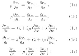
采用交错网格有限差分(Virieux, 1986; Luo and Schuster, 1990; 董良国等, 2000)求解方程(1a)-(1e). 2阶时间精度和2M阶空间精度的差分格式(以式(1a)为例)为

 (裴正林, 2004; Liu and Sen, 2009). Δt和h分别为时间和空间采样间隔, 上标k为时间节点索引数, 下标(i, j)为空间网格点索引数.
混合吸收边界条件是通过双程波波场和单程波波场加权平均实现的. 单程波方程的种类直接决定着混合吸收边界条件的吸收效果. 考虑到计算量和实现复杂度, 本文采用低阶Higdon单程波方程.
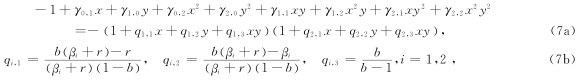
3.1 二阶Higdon单程波方程二阶Higdon位移单程波方程(Higdon, 1991)(以左边界为例)为
 , β1=1,β2=vP/vS, vP和vS分别为纵波和横波速度.
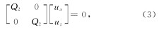
位移与速度、位移与应力的关系式(Levander, 1988)为
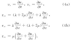
联立方程(3)和(4), 可得二阶Higdon速度-应力单程波方程为
为了获得较高的模拟精度, 采用下面的离散格式(Higdon, 1991)(以速度的水平分量为例):
左上角的离散格式可以通过加权平均左边界和上边界的格式得到, 形式如下(Liu and Sen, 2012):

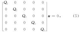
一阶Higdon位移单程波方程(Higdon, 1991)(以左边界为例)为

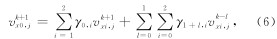
由上式可知, 此方程只对纵波有衰减作用, 不能很好地压制横波反射. 二阶Higdon单程波方程(方程(3))中第一项主要衰减纵波, 第二项主要衰减横波. 因此, 我们构造一个新的一阶Higdon单程波方程:
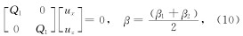
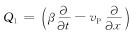 联立方程(4)和(10), 可得改进的一阶Higdon速度-应力单程波方程为
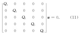
为了获得较高的模拟精度, 采用下面的离散格式(Higdon, 1991)(以速度的水平分量为例):
左上角的离散格式仍然可以通过加权平均左边界和上边界的格式得到, 形式如下:
将研究区域分成边界(区域III: A1, B1)、过渡(区域II: A2, A3, …, AN; B2, B3, …, BN; C1, C2, …, CN; D1, D2, …, DN)和内部(区域I)区域, 如图 1所示. 混合吸收边界条件的实现步骤如下:
(1)对区域I和区域II, 解双程波方程(1a)—(1e), 得到双程波波场: vtwox,vtwoz,τtwoxx,τtwozz,τtwoxz.
(2)对区域II和区域III, 解单程波方程(7)—(8)或(12)—(13), 得到单程波波场: vonex,vonez,τonexx,τonezz,τonexz.
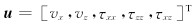
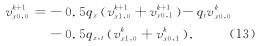
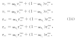
(3)对区域II, 将双程波波场和单程波波场加权平均得到最终的波场:

|
图 1混合吸收边界条件示意图(Liu and Sen, 2012) Fig. 1Illustration of hybrid absorbing boundary conditions (Liu and Sen, 2012) |
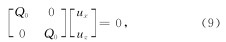
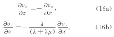
Lan和Zhang(2011)对数值模拟中处理自由边界的方法进行了详细研究, 主要有直接法和镜像法两种. 在直接法中, 满足如下方程(Hestholm and Ruud, 2000; 周竹生等, 2007):
由于直接求解方程(16)需要在自由表面附近进行降阶处理, 可能会导致不稳定或模拟精度不够, 因此直接法在实际中很少用.
镜像法(Levander, 1988; Liu and Sen, 2012)是另一种处理自由边界的方法. 它通过将自由表面两侧的应力场镜像反对称处理, 来满足边界上应力为零的条件. 该方法容易实现, 但缺少严格的理论支撑. 因此, 本文采用直接法和镜像法相结合的办法(Robertsson, 1996).
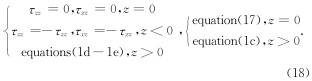
将方程(16b)带入方程(1c)得

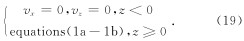
方程(1a)—(1b)中不包括τxx/z,因此自由表面上方不需要τxx.则应力更新公式如下:
这里分别采用均匀介质,高纵、横波速度比模型和Marmousi模型来验证混合吸收边界条件的有效性. 同时, 我们也从计算量、存储量及吸收效果等方面对混合吸收边界条件和PML边界条件进行比较.
首先设计一个均匀介质模型. 模型大小为2000 m ×2000 m, vP=4000 m/s, vS=2000 m/s, ρ=2100 kg/m3.空间网格大小为10 m×10 m, 时间步长为1 ms, 记录长度为2 s. 震源采用主频为15 Hz的Ricker子波, 位于模型中央, 施加在速度的水平分量上.
图 2为采用不同吸收边界条件得到的波场快照(图(a)、(b)、(c)和(d)中, 从上到下依次为x分量 和z分量, 从左到右依次为370 ms、620 ms和1000 ms 时的情况). 由图 2可知, 与无吸收边界条件相比, PML边界条件、混合一阶Higdon吸收边界条件和混合二阶Higdon吸收边界条件都能较好地吸收边界反射. 为了进一步比较, 图3a给出采用不同吸收边界条件时点(500 m, 250 m)处的振动图, 其中参考解为模型足够大时的情况. 由图可知, PML边界条件、混合一阶Higdon吸收边界条件和混合二阶Higdon吸收边界条件得到的结果与参考解相近. 图 3b是这三种边界条件模拟结果与参考解的振动误差图. 由图可见, 混合二阶Higdon吸收边界条件的吸收效果最好, 混合一阶Higdon吸收边界条件次之, PML边界条件最差.

|
图 2均匀介质模型中采用不同边界条件的波场快照 (a)无吸收边界;(b) PML边界条件; (c) 混合一阶Higdon吸收边界条件;(d) 混合二阶Higdon吸收边界条件. Fig. 2Snapshots by using different absorbing boundary conditions for a homogeneous model (a) Non-ABC;(b) PML ABC;(c) Hybrid 1st Higdon ABC;(d) Hybrid 2nd Higdon ABC. x- and z- components are from top to bottom, snapshots at 370 ms, 620 ms and 1000 ms from left to right. |

|
图 3均匀介质模型中采用不同吸收边界条件时点(500 m, 250 m)处的振动图(a)和误差图(b) 图(a)和(b)中, 从上到下依次为x分量和z分量. Fig. 3Records (a) and errors (b) at (500 m, 250 m) by using different absorbing boundary conditions for a homogeneous model (x- and z- components are from top to bottom) |
表 1和表 2分别为采用不同边界条件所需要的计算时间和存储量. 本次模拟是在计算机型号为HP p6615cn台式机(Intel(R) Core(TM) i3 处理器、2 GB 内存)上实现的. 由表可见, PML边界条件需要最长的计算时间和最大的存储空间, 混合二阶Higdon吸收边界条件居中, 混合一阶Higdon吸收边界条件消耗最少的计算机资源. 与常规的PML方法相比, 本文提出的两种混合Higdon吸收边界条件在占用较少的计算机资源的情况下能给出更好的吸收结果, 优势明显. 同时考虑计算效率和吸收效果, 下文只采用混合一阶Higdon吸收边界条件.
|
|
表 1不同吸收边界条件的计算时间 Table 1 The computational time by using different absorbing boundary conditions |
|
|
表 2不同吸收边界条件的存储量 Table 2The memory by using different absorbing boundary conditions |
在实际弹性波数值模拟中, 纵、横波速度比太大可能会引起不稳定现象(Hestholm, 2003; Opral and Zahradnik, 1999). 因此, 采用一个典型的高纵、横波速度比模型, 模型参数如图 4所示(Opral and Zahradnik, 1999; Liu and Sen, 2012). 空间网格大小为5 m×5 m, 时间步长为0.5 ms. 震源采 用主频为10 Hz的Ricker子波, 位于(500 m, 200 m) 处, 施加在速度的水平分量上. 图 5为采用不同边界条件时得到的波场快照. 由图可见, PML边界条件和混合一阶Higdon吸收边界条件都能吸收大部分的边界反射. 但在某些部位(箭头所指的位置), 采用混合一阶Higdon吸收边界条件时的边界反射要更弱.

|
图 4高纵、横波速度比模型(Liu and Sen, 2012) Fig. 4An elastic model with high vP/vS(Liu and Sen, 2012) |

|
图 5高纵、横波速度比模型中采用不同边界条件的波场快照 (a) 无吸收边界; (b) PML边界条件; (c) 混合一阶Higdon吸收边界条件.图(a)、(b)和(c)中, 从上到下依次为 x分量和z分量, 从左到右依次为2000 ms和4000 ms的波场快照. Fig. 5Snapshots by using different absorbing boundary conditions for an elastic model with high vP/vS (a) Non-ABC;(b) PML ABC;(c) Hybrid 1st Higdon ABC. x- and z- components are from top to bottom, snapshots at 2000 ms and 4000 ms from left to right. |
为了进一步验证本文提出的基于一阶弹性波方 程的混合吸收边界条件的有效性, 下面对Marmousi 模型(图 6)进行数值模拟. 空间网格大小为10 m×10 m, 时间步长为1 ms, 记录长度为4 s. 震源采用主频为15 Hz的Ricker子波, 位于(2500 m, 0 m)处, 施加在速度的水平分量上. 本例子中, 上边界采用自由边界条件. 图 7为采用不同边界条件的地面地震记录. 为了便于比较不同边界条件的吸收效果, 显示时采用自动增益控制. 由图 7b可见, 尽管PML边界条件可以吸收大量边界反射, 但当采用增益放大后, 可以看到一部分微弱的反射波(箭头所指的区域). 而图 7c中, 在相同的增益控制下难以看到边界反射, 表明混合吸收边界条件具有更好的吸收效果.

|
图 6 Marmousi vP模型(vS和ρ可以由经验公式求得) Fig. 6The Marmousi vP model (vS and ρ can be obtained by empirical formulas) |

|
图 7Marmousi模型中采用不同边界条件的地面地震记录 (a)无吸收边界条件; (b)PML边界条件; (c)混合一阶Higdon吸收边界条件. 图(a)、(b)和(c)中, 从左到右依次为x分量和z分量. Fig. 7Seismograms by using different absorbing boundary conditions for the Marmousi model (a) Non-ABC;(b) PML ABC;(c) Hybrid 1st Higdon ABC. x- and z- components are from left to right. |
稳定性是评价吸收边界条件好坏的重要指标. 这里将对本文提出的基于速度-应力方程的混合吸收边界条件的稳定性进行简要分析. 采用不同时刻内部区域的扰动能量大小来衡量边界条件的稳定性, 公式如下:
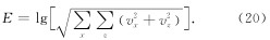
这里仍然以Marmousi模型为例来对比不同吸收边界条件的稳定性, 模型参数及观测系统参数同上. 图 8为采用不同边界条件时内部区域能量大小的变化曲线. 由图可见, 当时间较小时, 混合二阶Higdon 吸收边界条件、混合一阶Higdon吸收边界条件及PML边界条件都是稳定的. 随时间增大(大于2000 ms)时, 混合二阶Higdon吸收边界条件出现了不稳定现象, 这主要是由于一阶双程波方程和二阶单程波方程同时使用导致的. 而混合一阶Higdon边界条件仍然是稳定的.

|
图 8Marmousi模型中采用不同边界条件的内部区域能量曲线 Fig. 8Variation of energy in the inner area for the Marmousi model by using different absorbing boundary conditions |
为了进一步验证混合一阶Higdon吸收边界条件的有效性, 我们将计算时间增加至8 s, 并与Liu和Sen的方法(2012)进行了比较, 如图 9所示. 由于Liu和Sen的方法得到的是位移场, 而本文方法求得的是速度场, 两者大小有差异. 这里只对比其稳定性, 结论如下:
(1) 当过渡带点数较少或计算时间较大时, 现有的基于二阶位移-应力方程的混合吸收边界条件稳定性较差(如: N=2时, 4 s以后; N=5时, 7 s 以后).
(2) 当过渡带点数较少或计算时间较大时, 本文提出的混合一阶Higdon吸收边界条件稳定性较好(能量无增大趋势).
(3) 随着过渡带的点数增加, 稳定性逐渐变好, 但计算量相应增加.
本文提出的混合一阶Higdon吸收边界条件在各种试验中表现良好, 稳定可靠, 具有较好的应用 前景. 另外, 在构造混合吸收边界条件时, 单程波 方程的种类也很重要, 一方面影响边界条件的吸收效果, 另一方面也会对稳定性产生影响. 我们也尝试过用Clayton和Engquist(1977)单程波方程构造混合吸收边界条件, 但当纵、横波速度比较大时, 同样是不稳定的.

|
图 9Marmousi模型中采用混合一阶Higdon吸收边界条件和Liu和Sen方法的内部区域能量曲线 Fig. 9Variation of energy in the inner area for the Marmousi model by using our hybrid 1st Higdon and Liu and Sen′s absorbing boundary conditions |
本文推导了二阶和一阶Higdon速度-应力单程波方程; 提出基于一阶弹性波方程的混合吸收边界条件方法; 对多个模型进行了数值模拟与分析; 从计算时间、存储量和吸收效果等方面, 对混合吸收边界条件和常规的分裂PML边界条件进行了比较. 主要结论如下:
(1)在均匀,高纵、横波速度比及复杂介质的数值模拟中, 混合吸收边界条件都能够有效地吸收边界反射;
(2)与常规的PML方法相比, 混合吸收边界条件可以在消耗较少的计算时间和存储量的前提下, 给出更好的吸收效果;
(3)与混合二阶Higdon吸收边界条件相比, 混合一阶Higdon吸收边界条件具有更好的稳定性.
另外, 本文方法可以直接推广到二维或三维复杂介质(黏弹、各向异性)的数值模拟中, 也可以应用于涉及到波动方程数值求解的逆时偏移或全波形 反演中. 本文提出的吸收边界条件需要更少的计算机资源, 可以提高逆时偏移或全波形反演的计算效率.
| [1] | Bérenger J P. 1994. A perfectly matched layer for the absorption of electromagnetic waves. J. Comput. Phys., 114(2): 185-200, doi: 10.1006/jcph.1994.1159. |
| [2] | Cao S, Greenhalgh S. 1998. Attenuating boundary conditions for numerical modeling of acoustic wave propagation. Geophysics, 63(1): 231-243, doi: 10.1190/1.1444317. |
| [3] | Cerjan C, Kosloff D, Kosloff R, et al. 1985. A nonreflecting boundary condition for discrete acoustic and elastic wave equations. Geophysics, 50(4): 705-708. doi: 10.1190/1.1441945. |
| [4] | Clayton R, Engquist B. 1977. Absorbing boundary conditions for acoustic and elastic wave equations. Bull. Seism. Soc. Am., 67(6): 1529-1540. |
| [5] | Collino F, Tsogka C. 2001. Application of the perfectly matched absorbing layer model to the linear elastodynamic problem in anisotropic heterogeneous media. Geophysics, 66(1): 294-307, doi: 10.1190/1.1444908. |
| [6] | Dong L G, Ma Z T, Cao J Z, et al. 2000. A staggered-grid high-order difference method of one-order elastic wave equation. Chinese J. Geophys. (in Chinese), 43(3): 411-419. |
| [7] | Du Q Z, Li B, Hou B. 2009. Numerical modeling of seismic wavefields in transversely isotropic media with a compact staggered-grid finite difference scheme. Appl. Geophys., 6(1): 42-49, doi:10.1007/s11770-009-0008-z. |
| [8] | Du Q Z, Sun R Y, Zhang Q. 2011. Numerical simulation of three-component elastic wavefield in 2D TTI media in the condition of the combined boundary. Oil Geophys. Prosp. (in Chinese), 46(2): 187-195. |
| [9] | Engquist B, Majda A. 1977. Absorbing boundary conditions for numerical simulation of waves. Proc. Natl. Acad. Sci. USA, 74(5): 1765-1766. |
| [10] | Gao H, Zhang J. 2008. Implementation of perfectly matched layers in an arbitrary geometrical boundary for elastic wave modelling. Geophys. J. Int., 174(3): 1029-1036, doi: 10.1111/j.1365-246X.2008.03883.x. |
| [11] | Heidari A H, Guddati M N. 2006. Highly accurate absorbing boundary conditions for wide-angle wave equations. Geophysics, 71(3): S85-S97, doi: 10.1190/1.2192914. |
| [12] | Hestholm S. 2003. Elastic wave modeling with free surfaces: Stability of long simulations. Geophysics, 68(1): 314-321, doi: 10.1190/1.1543217. |
| [13] | Hestholm S O, Ruud B. 2000. 2D finite-difference viscoelastic wave modelling including surface topography. Geophys. Prospect., 48(2): 341-373, doi: 10.1046/j.1365-2478.2000.00185.x. |
| [14] | Higdon R L. 1991. Absorbing boundary conditions for elastic waves. Geophysics, 56(2): 231-241, doi: 10.1190/1.1443035. |
| [15] | Hu W Y, Abubakar A, Habashy T M. 2007. Application of the nearly perfectly matched layer in acoustic wave modeling. Geophysics, 72(5): SM169-SM175, doi: 10.1190/1.2738553. |
| [16] | Komatitsch D, Martin R. 2007. An unsplit convolutional perfectly matched layer improved at grazing incidence for the seismic wave equation. Geophysics, 72(5): SM155-SM167, doi: 10.1190/1.2757586. |
| [17] | Komatitsch D, Tromp J. 2003. A perfectly matched layer absorbing boundary condition for the second-order seismic wave equation. Geophys. J. Int., 154(1): 146-153, doi: 10.1046/j.1365-246X.2003.01950.x. |
| [18] | Kosloff R, Kosloff D. 1986. Absorbing boundaries for wave propagation problems. J. Comput. Phys., 63(2): 363-376, doi: 10.1016/0021-9991(86)90199-3. |
| [19] | Lan H, Zhang Z. 2011. Comparative study of the free-surface boundary condition in two-dimensional finite-difference elastic wave field simulation. J. Geophys. Eng., 8(2): 275-286, doi:10.1088/1742-2132/8/2/012. |
| [20] | Levander A R. 1988. Fourth-order finite-difference P-SV seismograms. Geophysics, 53(11): 1425-1436, doi: 10.1190/1.1442422. |
| [21] | Liu Y, Sen M K. 2009. An implicit staggered-grid finite-difference method for seismic modelling. Geophys. J. Int., 179(1): 459-474, DOI: 10.1111/j.1365-246X.2009.04305.x. |
| [22] | Liu Y, Sen M K. 2010. A hybrid scheme for absorbing edge reflections in numerical modeling of wave propagation. Geophysics, 75(2): A1-A6, doi: 10.1190/1.3295447. |
| [23] | Liu Y, Sen M K. 2012. A hybrid absorbing boundary condition for elastic staggered-grid modelling. Geophys. Prospect., 60(6): 1114-1132, doi: 10.1111/j.1365-2478.2011.01051.x. |
| [24] | Luo Y, Schuster G. 1990. Parsimonious staggered grid finite-difference of the wave equation. Geophys. Res. Lett., 17(2): 155-158, doi: 10.1029/GL017i002p00155. |
| [25] | Martin R, Komatitsch D. 2009. An unsplit convolutional perfectly matched layer technique improved at grazing incidence for the viscoelastic wave equation. Geophys. J. Int., 179(1): 333-344, doi: 10.1111/j.1365-246X.2009.04278.x. |
| [26] | Martin R, Komatitsch D, Gedney S D. 2008. A variational formulation of a stabilized unsplit convolutional perfectly matched layer for the isotropic or anisotropic seismic wave equation. Comput. Model. Eng. Sci., 37(3): 274-304, doi: 10.3970/cmes.2008.037.274. |
| [27] | Opral I, Zahradnik J. 1999. From unstable to stable seismic modelling by finite-difference method. Phys. Chem. Earth, Part A, 24(3): 247-252, doi: 10.1016/S1464-1895(99)00026-5. |
| [28] | Pei Z L. 2004. Numerical modeling using staggered-grid high-order finite-difference of elastic wave equation on arbitrary relief surface. Oil Geophys. Prosp. (in Chinese), 39(6): 629-634. |
| [29] | Robertsson J O A. 1996. A numerical free-surface condition for elastic/viscoelastic finite-difference modeling in the presence of topography. Geophysics, 61(6): 1921-1934, doi: 10.1190/1.1444107. |
| [30] | Tian X, Kang I B, Kim G Y, et al. 2008. An improvement in the absorbing boundary technique for numerical simulation of elastic wave propagation. J. Geophys. Eng., 5(2): 203-209, doi:10.1088/1742-2132/5/2/007. |
| [31] | Virieux J. 1986. P-SV wave propagation in heterogeneous media: Velocity-stress finite-difference method. Geophysics, 51(4): 889-901, doi: 10.1190/1.1442147. |
| [32] | Wang T, Tang X. 2003. Finite-difference modeling of elastic wave propagation: A nonsplitting perfectly matched layer approach. Geophysics, 68(5): 1749-1755, doi: 10.1190/1.1620648. |
| [33] | Wang X M, Zhang H L, Wang D. 2003. Modelling of seismic wave propagation in heterogeneous poroelastic media using a high-order staggered finite-difference method. Chinese J. Geophys. (in Chinese), 46(6): 842-849. |
| [34] | Yang D H. 2002. Finite element method of the elastic wave equation and wavefield simulation in two-phase anisotropic media. Chinese J. Geophys. (in Chinese), 45(4): 575-583. |
| [35] | Zeng Y, He J, Liu Q. 2001. The application of the perfectly matched layer in numerical modeling of wave propagation in poroelastic media. Geophysics, 66(4): 1258-1266, doi: 10.1190/1.1487073. |
| [36] | Zhang L X, Fu L Y, Pei Z L. 2010. Finite difference modeling of Biot's poroelastic equations with unsplit convolutional PML and rotated staggered grid. Chinese J. Geophys. (in Chinese), 53(10): 2470-2483, doi: 10.3969/j.issn.0001-5733.2010.10.021. |
| [37] | Zhou Z S, Liu X L, Xiong X Y. 2007. Finite-difference modelling of Rayleigh surface wave in elastic media. Chinese J. Geophys. (in Chinese), 50(2): 567-573. |
| [38] | Zhang J F, Liu T L. 1999. P-SV-wave propagation in heterogeneous media: grid method. Geophys. J. Int., 136(2): 431-438, doi: 10.1111/j.1365-246X.1999.tb07129.x. |
| [39] | Zhou H, McMechan G A. 2000. Rigorous absorbing boundary conditions for 3-D one-way wave extrapolation. Geophysics, 65(2): 638-645, doi: 10.1190/1.1444760. |
| [40] | 董良国,马在田,曹景忠等.2000.一阶弹性波方程交错网格高阶差分解法.地球物理学报,43(3):411-419. |
| [41] | 杜启振,孙瑞艳,张强.2011.组合边界条件下二维三分量TTI介质波场数值模拟.石油地球物理勘探,46(2):187-195. |
| [42] | 裴正林.2004.任意起伏地表弹性波方程交错网格高阶有限差分法数值模拟.石油地球物理勘探,39(6):629-634. |
| [43] | 王秀明,张海澜,王东.2003.利用高阶交错网格有限差分法模拟地震波在非均匀孔隙介质中的传播.地球物理学报,46(6):842-849. |
| [44] | 杨顶辉.2002.双相各向异性介质中弹性波方程的有限元解法及波场模拟.地球物理学报,45(4):575-583. |
| [45] | 张鲁新,符力耘,裴正林.2010.不分裂卷积完全匹配层与旋转交错网格有限差分在孔隙弹性介质模拟中的应用.地球物理学报,53(10):2470-2483,doi:10.3969/j.issn.0001-5733.2010.10.021. |
| [46] | 周竹生,刘喜亮,熊孝雨.2007.弹性介质中瑞雷面波有限差分法正演模拟.地球物理学报,50(2):567-573. |