 2013, Vol. 56


2. 中国科学院大学, 北京 100049
2. University of Chinese Academy of Sciences, Beijing 100049, China
地震波数值模拟是研究地震波传播问题的重要手段,在研究地震波在地球内部的传播规律和实际资料的处理与解释方面均能发挥着重要作用.目前,比较常用的方法有,有限差分法[1-7]、伪谱法[8-10]、有限元法[11-32]、谱元法[33-39]、有限体积法[40]等.有限差分法具有编程简单,计算效率高等特点,但是有严重的数值频散且难以处理起伏地表和自由边界条件[1-7].伪谱法[8-10]是一种全局的方法,具有计算精度高和数值频散小的特点,但是在强非均匀介质的边界处会出现数值不稳定现象[8-10],它与有限差分法一样,具有难以处理起伏地表和自由边界条件之不足.有限元法[11-32]克服了大部分这些缺点,可适应于任意几何模型,能够自然地满足自由边界条件(地表的牵引力为零),但仍为低阶的近似,具有计算量大和占用内存大等缺点.谱元法[33-40]与有限元法类似,是高阶的有限元法,并具有较高的计算精度,采用Gauss-Lobatto-Legendre积分以得到对角的质量矩阵提高计算效率,但计算量和内存占用量仍然较大.为了满足稳定性条件,用谱元法进行地震波数值模拟时所需要的时间采样间隔会随着Legendre多项式的阶数的增高而显著减小,导致计算量随之呈指数增长[33-34].
有限元法由于能够很好地刻画复杂介质与结构的几何模型和自然地满足自由边界条件,故在地震学研究中也得到应用.1984年Marfurt[18]进行了传统有限差分法和有限元法精度的对比研究.崔力科等[24]对有限元数值解的稳定性、精确度等问题做了详细研究,求解了无阻尼地震模型、三维阻尼地震模型的有限元数值解以及有限元偏移成像技术.王尚旭[25](1990)利用有限元方法研究了双相各向同性介质中弹性波的传播规律.Padovani(1994)等[18]研究了地震波有限元模拟中的低阶有限元和高阶有限元法的精度.周辉和徐世浙[26](1997)对各向异性介质中波动方程的有限元数值解的稳定性做了深入探讨.Sarma[41](1999)研究了弹性波传播的有限元模拟的衰减吸收边界条件问题,给出了应用于有限元法的无反射边界条件.柯本喜等[27](2001)使用三角形和四边形联合有限元法,求解起伏地表下的标量波波动方程.张美根和王妙月[28](2002)实现了各向异性介质的有限元正演模拟、有限元偏移技术和有限元参数反演技术.张剑锋等[29](2002)采用集中质量矩阵实现了各向异性介质的弹性波有限元数值解.马德堂和朱光明[31](2004)把有限元法和伪谱法相结合,求解起伏地表下的弹性波动方程.黄自萍[32]等(2004)采用区域分解算法,把有限元法与有限差分法相结合进行起伏地表的数值模拟.
有限元方程形成的刚度矩阵是大型的稀疏矩阵,完全存储需要巨大的内存空间.本文对刚度矩阵采用压缩存储行(CSR)格式[42-45]进行存储.由于在时间推演过程中,只涉及到刚度矩阵与位移向量的乘积,因此只需存储非零元素以节省计算机内存空间、且同时减少浮点运算.经典的有限元方程中形成的质量矩阵是非对角的一致质量矩阵,利用质量守恒原理,把单元所有质量集中在单元节点上,以形成对角的集中质量矩阵[19, 46-50]以替代一致质量矩阵,从而显式(显式有限元法)地递推避免求解大型稀疏方程组,提高了有限元法数值模拟的计算效率.在时间离散上采用保能量的Newmark格式以改善时间差分精度[51-54].在地震学中,最近发展起来的谱元法[33-40]具有计算精度高的特点,但其计算量较大.
人工截断边界条件是波场模拟的一个重要方面,前人为此做了大量的研究工作,并发展了多种边界条件[55-95],其中以完全匹配吸收边界条件的吸收效果最佳.为此本文在有限元法中发展了PML吸收边界条件.在1994年,Berenger针对电磁波传播问题,引进了一种高效的最佳匹配层(perfectly matched layer,简称PML)吸收边界条件[61],并在理论和模型算例上证明了该方法可以较好地吸收来自各个方向和各个频率的波[62-63],且不会产生明显的边界虚假反射波.后来,Chew和Liu.[63]将PML技术引入到弹性波的数值模拟中.Collino和Tsogka[65]进一步把PML应用到各向异性非均匀介质的地震波的波场模拟中;Festa[67]针对各向同性弹性介质情况,对PML离散波动方程的稳定性进行了详细讨论,并推导了PML吸收边界条件的理论反射系数公式;Becache et al.[68]在理论上讨论了PML在各向异性情况下的稳定性问题.目前,PML已经应用到很多领域,在声波[69-72]、弹性波[73-74]、黏弹性介质[75]、双相孔隙弹性介质[76-77],各向异性介质[78],面波频散[79-80]等的数值模拟中并得到了广泛的应用,并且PML不断地得到发展[81-94]和改进[64, 95].在人工截断边界上,以变分[90]的形式将PML吸收边界引入到有限元的方程组中去,取得了良好的吸收效果.
本文首先在复数伸展坐标下,构建带PML吸收的二阶弹性波动方程,通过在频率域引入4个中间变量,然后将其变换到时间域以获取精确的表达式,并组合到有限元方程组中得到相应的变分形式.对刚度矩阵采用压缩存储行(CSR)格式,以减少计算量并节省内存;采用质量集中技术得到对角的质量矩阵以提高有限元法(显式有限元)的计算效率;时间离散采用保能量的Newmark算法以提高有限元法的计算精度.接着,用拉梅问题[96]测试显式有限元法的计算精度和本文构建的PML吸收边界条件的有效性.最后,为了测试显式有限元法在起伏地表模型中对面波和体波的计算精度(考虑地形对波场的影响)[97-102],设计一个起伏地表模型,在计算效率和计算精度方面将其与谱元法进行对比研究.
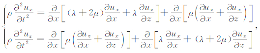
2 复数伸展坐标下的弹性波动方程及其PML吸收边界条件Chew和Liu(1996)将PML吸收边界条件表述为在频率域引入了伸展坐标系.为此,在复数伸展坐标系下构建二阶弹性波动方程的PML吸收边界条件. 2.1复数伸展坐标下的弹性波波动方程二维各向同性介质中的弹性波波动方程[49]为
|
(1) |
其中,ρ(x,z)为介质的密度;ux(x,z)和uz(x,z)分别是质点在水平方向和垂直方向的位移;t是时间;λ和μ为拉梅常数.
复数伸展坐标下的弹性波动方程为

|
(2) |
其中,i为虚数单位;ω为角频率;Ux,Uz分别为ux,uz关于时间的傅里叶变换;dx(x),dz(z)为衰减系数,经验值[65]dx(x)=-(n+1)log(R)Vp/(2δ)·(x/δ)n,δ为PML层的厚度;x为吸收层到计算区域边界的距离;n为控制衰减系数衰减快慢的常数,一般取2~3;R为理论反射系数,一般取1.0×10-2~10-6.
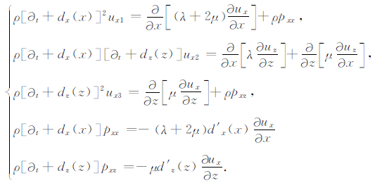
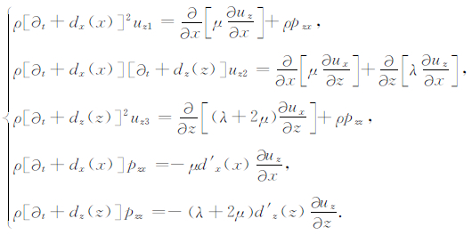
2.2 PML吸收边界条件将公式(2)中的两式分别分裂为3项,并变换到时间域得到如下方程组:
|
(3) |
|
(4) |
其中,ux=ux1 +ux2 +ux3,uz=uz1 +uz2 +uz3,pxx,pxz,pzx,pzz为引入的中间变量.d′x(x)=∂dx(x)/∂x,d′z(z)=∂dz(z)/∂z以变分形式表示在上述方程组中(见(9),(10)式).(3)和(4)式为含PML吸收边界条件的弹性波波动方程,可以在时间上递推.在计算区域内,dx(x)=dz(z)=0,(3)和(4)式退化为无衰减的波动方程;在吸收层内,dx(x)≠0,dz(z)≠0用以减弱人工边界处的虚假反射波.本文构建的PML吸收边界条件仅需将位移分量分裂成3项,相比于Komatitsch和Tromp(2003)构建的PML吸收边界条件把位移在全局分裂成5项,在不降低计算精度的前提下节省内存空间.
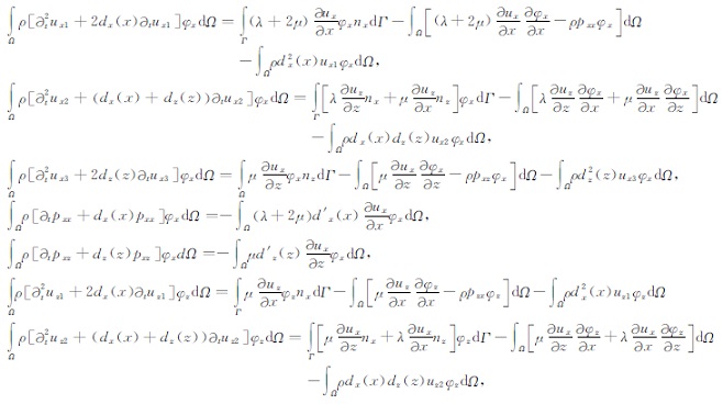
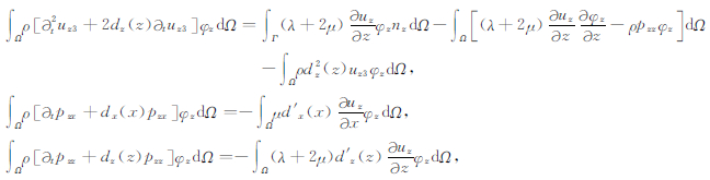
2.3 有限元方程组方程(3)和(4)相应的弱形式为
|
(5) |
|
(6) |
其中,Ω,Γ分别是计算区域及其边界;n=(nx,nz)T为计算区域的边界的外法线向量;φ=(φx,φz)T为虚位移向量.在PML边界上利用位移为0的Dirichlet边界条件,上边界处理为自由边界条件.
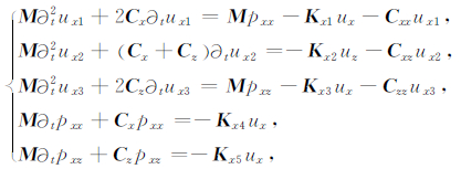
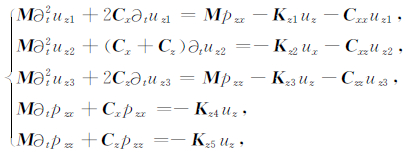
形成的有限元方程组为
|
(7) |
|
(8) |
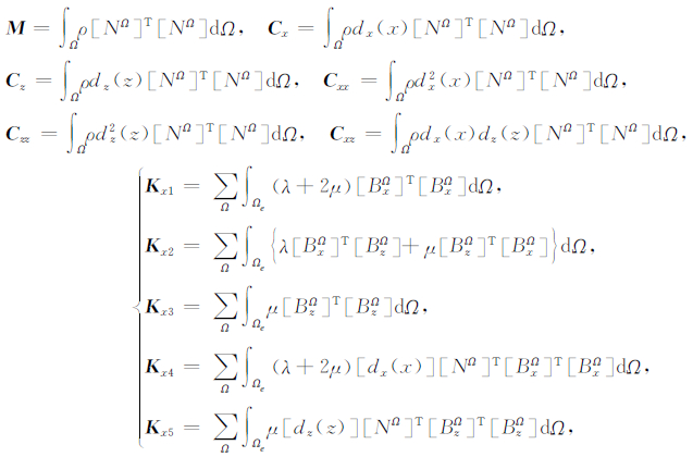
其中,
|
(9) |

|
(10) |
[NΩ]是计算区域内的形函数;[BxΩ]和[BzΩ]分别是在计算区域内形函数关于x和z的导数;
(7)和(8)各式具有的一般形式为
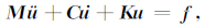
|
(11) |
其中,M为质量矩阵,C为阻尼矩阵,f为荷载向量;
有限元形成的刚度矩阵是一个大型的稀疏矩阵,全部存储需要很大的内存空间.本文采用稀疏矩阵的压缩存储行(CSR)格式只需存储其非零元素,故大大减少了所需存储空间.在时间推演过程中,由于只涉及到矩阵与向量的乘积,因而这种稀疏存储格式同时可以减少计算量.对于稀疏矩阵只需用三个一维数组存储其非零元素[42-45].
3.2 集中质量矩阵
经典有限元方程组中的质量矩阵为非对角的,称为一致质量矩阵.根据质量守恒原理,把单元上的质量集中分配在单元节点上,将一致质量矩阵转化为对角的集中质量矩阵[46-50].对于一致质量矩阵M=mij,其中
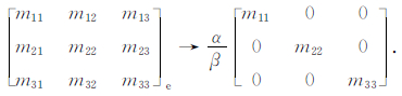
|
(12) |
当然,用集中质量矩阵代替一致质量矩阵是一种近似计算,本文将在4.1-4.2节中验证其计算精度.由于集中质量矩阵是对角的,可以与谱元法一样在时间上进行显式的递推(因而称为显式有限元法).不再像经典有限元方法,需要求解大型的稀疏代数方程组,故大大地提高了计算效率.在附录A中,我们讨论了本文所采用的集中质量矩阵与一致质量矩阵之间的差异,其频散分析参见文献[103-106].
3.3 时间离散--Newmark算法
Newmark算法[51]最初由Newmark提出(1959),是一种时间积分算法,具有保能量的特性(当β=0,γ=1/2时).该算法将点

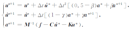
|
(13) |
其中,n为时间步数,a为加速度.当γ<1/2是能量消耗的;γ>1/2是能量增长的;当且仅当β=0,γ=1/2为保能量的.
4 数值算例 4.1 拉梅问题用拉梅问题[96]对显示有限元法的计算精度进行测试,模型尺寸为2000m×1000m的均匀介质;纵波速度2000m/s,横波速度为1150 m/s,密度为2000kg/m3.震源为15 Hz的雷克子波(垂向集中力源),位于点(1000 m,-50 m)处.显式有限元法的计算区域和吸收层均被剖分成非结构化的三角形网格,最大边长为10.39m,最小边长为1.10m,共有170581个单元,86347个节点(含边界),采用一阶线性插值;吸收层厚度为100 m(谱元法仅有两个单元),理论反射系数R取5.0×10⁻²;上边界为自由边界条件,左、右、下边界为PML吸收边界条件.时间采样为0.5 ms,共模拟到2.5s.谱元法的计算区域和吸收层均被剖分成结构化的四边形网格,边长为50m,共44×22个单元,采用7阶插值,形成47895个Gauss-Lobatto-Legendre积分节点(含边界);其他参数与有限元法相同.
图 1(a-b)为检波点(1800m,0m)处的水平位移分量(a)和垂直位移分量(b)的地震记录;图 1(c-d)为检波点(2000 m,0 m)处的地震记录.其中,红线为解析解,绿线为7阶谱元法的计算结果,蓝线为显式有限元法计算的结果.从图 1可以看到,显式有限元法和谱元法(SEM)都能对体波和面波进行较精确的模拟.同时,本文构建的PML吸收边界条件也取得了良好的吸收效果,没有来自人工截断边界的明显的虚假反射波.

|
图 1 检波点(1800m,0m)和(2000m,0m)处的地震记录 (a)和(b)分别是(1800m,0m)处的x和z位移分量;(c)和(d)分别是(2000m,0m)处的x和z位移分量;红线为解析解,绿线为7阶谱元法的结果,蓝线为显式有限元法的结果. Fig. 1 Seismic records from receivers at point (1800m, 0m) and (2000m, 0m) (a, b) are the seismic records in x-and z-direction from receiver at point (1800 m, 0 m), respectively; (c, d) are the seismic records in x-and z direction from receiver at point (2000 m, 0 m), respectively. Red lines denote the analytical solution; green lines denote results calculated by the SEM with polynomials of degree 7; blue lines denote the results calculated by the explicit FEM. |
图 2是显式有限元法在0~2.5s时间段内的动能、势能和总能量变化曲线.在0.1s到0.6s时间段内,地震波的动能、势能和总能量随着时间几乎是守恒的.在0.58s之后,体波逐渐传出计算区域,总能量递减近5130J左右;在1.0s之后,面波也逐渐传出计算区域,能量迅速衰减至0.可见,PML吸收边界条件是有效的.

|
图 2 能量随时间的变化曲线 红线为动能, 蓝线为势能, 绿线是总能量. Fig. 2 Curves of energy evolution with the growing of time Red line for the kinetic energy; Blue line for the potential energy; Green line for the total energy. |
为了验证显式有限元法在复杂模型中的计算精度,以及本文构建的PML吸收边界条件在复杂模型中的吸收效率,用图 3所示的起伏地表模型进行测试.模型横向长度为3000m,纵向延伸至1000m深,地表最大高程为400m.模型上层介质的纵波速度为2000m/s,横波速度为1300 m/s,质量密度为2000kg/m3;下层纵波速度为2800 m/s,横波速度为1473 m/s,质量密度为2500kg/m3.震源位于(1500m,0m)处,为15Hz的雷克子波(爆炸源).

|
图 3 起伏地表模型 三角形代表检波器的位置. Fig. 3 A model with irregular topography Triangles denote the receivers. |
显式有限元法的计算区域和吸收层均被剖分成非结构化的三角形网格,最大边长为10.41m,最小边长为2.18m,共有324577个单元,163497个节点(含边界),采用一阶线性插值;吸收层厚度为200m,理论反射系数R取5.0×10⁻²,时间采样间隔为0.5ms,共模拟到6s.谱元法的计算区域和吸收层均被剖分成非结构化的四边形网格,最大边长为89.67m,最小边长为10.07 m,共2719个单元,形成134373个Gauss-Lobatto-Legendre积分节点(含边界);采用7阶插值,由于稳定性要求,时间采样间隔取为0.1ms.由于谱元法具有较高的精度,其数值解是可靠的.为此,以谱元法的数值解作为参考以考查显式有限元法的计算精度.
图 4分别是0.4s(a-b)、0.8s(c-d)和1.0s(e-f)时刻的波场快照图.其中,(a,c,e)是谱元法模拟的结果;(b,d,f)是显式有限元模拟的结果,两者的主要波场信息是非常一致的.从图中可见,0.4s时刻谱元法和显式有限元法的波场快照并无差异,然而随着时间的推移,波场快照上有微小的差异(箭头所指示的位置).追踪波场快照可以发现,这些差异均为来自于与起伏地表和物性界面有关的反射波等.

|
图 4 不同时刻垂直位移分量的波场快照 (a,c,e)谱元法;(b,d,f)显式有限元法.从上到下依次是0.4 s,0.8 s和1.0 s时刻的波场快照. Fig. 4 Snapshots at different time instant of the vertical component of displacement Left column photos: the SEM (a, c, e); Right column photos: the explicit FEM (b, d, f). From top to bottom, snapshots at 0.4 s, 0.8 s and 1.0 s time-instant are shown, respectively. |
图 5分别是谱元法(a)和显式有限元法(b)计算的垂直位移分量合成地震图.从合成地震图可见,显式有限元法与谱元法模拟得到的主要波场信息是非常一致的,但是从波场快照上能发现微小的差异.

|
图 5 垂直位移的合成地震图 (a)谱元法;(b)显式有限元法. Fig. 5 Synthetic seismogram of the vertical component of displacement (a) The SEM; (b) The explicit FEM. |
图 6是检波点(2500 m,316.5 m)处的水平和垂直位移分量的地震记录.从图中可以看到,在短时程内,显式有限元法与谱元法的结果非常一致,随着时间的推进,两者的偏差增大(2.5s以后);但是两者的主要波场信息是非常一致的.两者在2.5s之前的振幅差异可能是由于所使用的多项式的阶数(即计算精度)不同造成的,而尾波的差异可能主要是起伏地表和物性界面的网格离散的差异(谱元法使用的网格更粗)导致的,当然计算精度的差异也可能有一定的贡献(见图 4).

|
图 6 检波点(2500 m,316. 5 m)处的地震记录 (a)水平位移;(b)垂直位移;绿线为谱元法,红线为显式有限元法. Fig. 6 Seismic records from receiver at point (2500 m, 316. 5 m) (a) Horizontal displacement component; (b) Vertical displacement component. Green lines: the SEM; Red lines: the explicit FEM. |
本文对显式有限元法与谱元法的刚度矩阵均采用上述的CSR稀疏存储格式.分别编制显式有限元法和谱元法的串行程序,并在同一台电脑(lenovo Think Centre M8300t)上运行.
表 1统计了显式有限元法和谱元法计算4.1节中的均匀模型和4.2节中带起伏地表的层状模型的CPU耗时以及平均每步耗时.从表 1可见,显式有限元法的计算速度是7阶谱元法的2倍左右,这个比值在均匀模型中约为1.5.
|
|
表 1 CPU耗时统计 Table 1 The statistic for CPU time consuming |
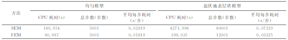
表 2是对上述两个模型的内存占用情况的统计.为了使两者达到相当的计算精度,显式有限元法需要的网格更细,因而显式有限元法的质量矩阵所消耗的内存量大于谱元法的.谱元法在单元内部需要插入GLL节点,随着阶数的增高,内存占用量呈指数增加[33-34],因而它的刚度矩阵的内存消耗远远大于显式有限元法的.从总的内存占用情况来看,谱元法的内存消耗大于显式有限元法,即显式有限元法的内存占用量仅为谱元法(7阶)的1/4~1/6.显见,谱元法是一种计算量和内存需求密集型的算法,因而计算效率低于显式有限元法,但是在长时程的数值模拟中它的计算精度高于显式有限元法的.然而,权衡考虑计算效率和计算精度,对于不考虑精细结构的大尺度模拟,显式有限元法是一种较好的方法.
|
|
表 2 内存占用情况统计 Table 2 The statistic for memory occupation |

正如上述,在短时程数值模拟中,显式有限元法可以获得与谱元法相当的结果.但是,随着时间的推移,两者的差异增大.我们分析,导致这种差异的原因有如下几个:(1)两者所使用的网格的差异,有限元法使用三角形网格,而谱元法使用四边形网格,而且四边形网格的边长远远大于三角形网格的,这在自由地表和内部的物性边界的离散上存在较大的差异;(2)两者的计算精度的差异;(3)来自边界的弱反射等.其中,第一个原因可能是主要的,由于两者使用的网格差异,使得地表和物性界面附近的波场采样点不能完全重合.特别是,四边形网格刻画起伏地表不如三角形网格灵活(水平地表不存在这种差异,见图 1).随着时间的推移,致使来自尖锐网格点的散射波,以及由于局部网格离散的不同引起的反射波场的差异被体现出来.当然,第二个原因也有一定的贡献,由于两者的计算精度的差异,也会导致这种偏差,这体现在2.5s以前的记录上.为了减小两者的差异,可以提高有限元法的插值阶数,减小谱元法在起伏地表和内部物性界面附近的网格剖分的尺寸.当然,这会成倍地增加谱元法模拟的总时间,因为使用的网格更精细,稳定性条件更苛刻,时间采样间隔需要取得更小.
6 结论本文构建了二阶弹性波动方程变分形式的PML吸收边界条件,并对有限元法和谱元法的刚度矩阵采用压缩存储行(CSR)格式进行稀疏存储,在时间离散上采用Newmark积分算法.数值试验表明,本文提出的PML吸收边界条件能对来自边界的虚假反射波进行较好的吸收(谱元法中仅需两个单元),而不产生明显的反射波.谱元法和显式有限元法的对比实验表明,在计算精度相近的情况下,显式有限元法的计算速度为谱元法(7阶)的2倍左右,而内存占用量仅为谱元法(7阶)的1/4~1/6.由于谱元法使用高阶的多项式,具有较高的精度;而显式有限元法使用低阶多项式,且采用质量集中这种近似获取对角矩阵以提高计算效率,在长时程的计算中两者有一定的差异.相比于谱元法所使用的四边形网格,显式有限元法使用的三角形网格则更加灵活,并能够非常容易地刻画更加复杂的几何模型.权衡考虑两者的计算效率和计算精度,对于不考虑精细结构的大尺度模拟,显式有限元法不失为一种很好的近似.
附录A一致质量矩阵与集中质量矩阵的关系如下:

|
(A1) |
(1)在有限元中,每个单元中的密度是均匀的,一致质量矩阵的各个元素有如下的关系:
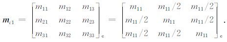
|
(A2) |
其中,m11=ρJ/6,ρ为质量密度,J为三角形的面积.
对于一个单元,其质量矩阵为表达式(A2),则相对误差矩阵为:
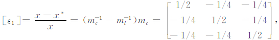
|
(A3) |
(2)对于两个单元,其质量矩阵为(当ρ2J2/ρ1J1=γ21):
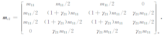
|
(A4) |
相对误差矩阵为:
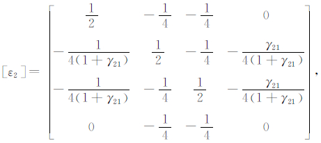
|
(A5) |
其中,J为雅可比矩阵的行列式的绝对值,即三角形单元的面积.
(3)对于三个单元,其质量矩阵为(当ρ3J3/ρ1J1=γ31):
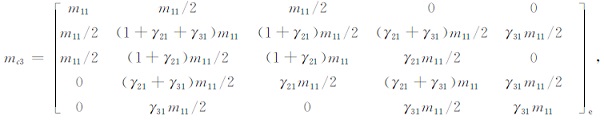
|
(A6) |
其误差矩阵
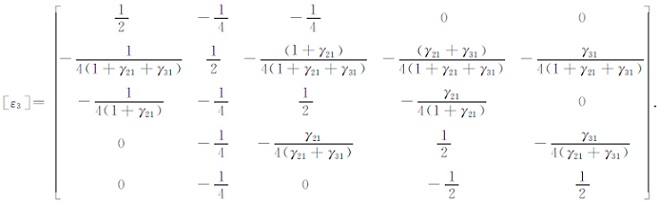
|
(A7) |
可见,误差矩阵的每行元素的求和为0,这意味着如果剖分的网格尺寸较小,误差会相互抵消.因此,显式有限元的计算精度与网格尺寸有关,网格尺寸越小越精确.
| [1] | Alford R M, Kelly K R, Boore D. Accuracy of finite-difference modeling of the acoustic wave equation. Geophysics , 1974, 39(6): 834-842. DOI:10.1190/1.1440470 |
| [2] | Kelly K R, Ward R W, Treitel S, et al. Synthetic seismograms: a finite-difference approach. Geophysics , 1976, 47(1): 2-27. |
| [3] | Marfurt K J. Accuracy of finite-difference and finite-element modeling of the scalar and elastic wave equations. Geophysics , 1984, 49(5): 533-549. DOI:10.1190/1.1441689 |
| [4] | Virieux J. SH-wave propagation in heterogeneous media: velocity-stress finite-difference method. Geophysics , 1984, 49(11): 1933-1942. DOI:10.1190/1.1441605 |
| [5] | Virieus J. P-SV wave propagation in heterogeneous media: velocity-stress finite-difference method. Geophysics , 1986, 51(4): 889-901. DOI:10.1190/1.1442147 |
| [6] | Graves R W. Simulating seismic wave propagation in 3D elastic media using staggered-grid finite differences. Bull. Seismol. Soc. Am. , 1996, 86(4): 1091-1106. |
| [7] | Bohlen T, Saenger E H. Accuracy of heterogeneous staggered-grid finite-difference modeling of Rayleigh waves. Geophysics , 2006, 71(4): T109-T115. DOI:10.1190/1.2213051 |
| [8] | Fornberg B. The pseudospectral method: accurate representation of interfaces in elastic wave calculations. Geophysics , 1988, 53(5): 625-637. DOI:10.1190/1.1442497 |
| [9] | Carcione J M, Wang P J. A Chebyshev collocation method for the wave equation in generalized coordinates. Comp. Fluid Dyn. J. , 1993, 2: 269-290. |
| [10] | Tessmer E, Kosloff D. 3-D elastic modeling with surface topography by a Chebyshev spectral method. Geophysics , 1994, 59(3): 464-473. DOI:10.1190/1.1443608 |
| [11] | Lysmer J, Drake L A. A Finite Element Method for seismology. // Bolt B ed. Methods in Computational Physics. New York: Scademic Press, 1972. |
| [12] | Smith W D. The application of finite element analysis to body wave propagation problems. Geophysical Journal of the Royal Astronomical Society , 1975, 42(2): 747-768. |
| [13] | Smith W D. Free oscillations of a laterally heterogeneous earth: A finite element approach to realistic modelling. Physics of the Earth and Planetary Interiors , 1980, 21(2-3): 75-82. DOI:10.1016/0031-9201(80)90059-X |
| [14] | Kuo J T, Teng Y C. Three-dimensional finite element modeling of acoustic and elastic waves. // 52nd Ann. Internat. Mtg. Soc. of Exploration Geophysicist, Session: RW1. 6, 1982. |
| [15] | Hughes T J R. The Finite Element Method: Linear Static and Dynamic Finite Element Analysis. Englewood Cliffs: Prentice Hall Inc., 1987 . |
| [16] | Marfurt K J. Analysis of higher order finite-element methods: numerical modeling of seismic wave propagation. Society of Exploration Geophysicist, 1990. |
| [17] | Kelly K R, Marfurt K J. Numerical modeling of seismic wave propagation. Geophysics Reprint Series, Society of Exploration Geophysicists Reprint Series, No. 13, 1990: 520. |
| [18] | Padovani E, Priolo E, Seriani G, et al. Low and high order finite element method: experience in seismic modeling. J. Comp. Acous. , 1994, 2(4): 371-422. DOI:10.1142/S0218396X94000233 |
| [19] | Richter G R. An explicit finite element method for the wave equation. Appl. Num. Math. , 1994, 16(1-2): 65-80. DOI:10.1016/0168-9274(94)00048-4 |
| [20] | Zhu J L. 2.5-D finite element seismic modelling: 64th Ann. Internat. Mtg. Soc. of Exploration. Geophysicist , 1994: 1375-1377. |
| [21] | Komatitsch D, Coutel F, Mora P. Tensorial formulation of the wave equation for modelling curved interfaces. Geophys. J. Int. , 1996, 127(1): 156-168. DOI:10.1111/gji.1996.127.issue-1 |
| [22] | Moser F, Jacobs L J, Qu J M. Modeling elastic wave propagation in waveguides with the finite element method. NDT & E International , 1999, 32(4): 225-234. |
| [23] | Kay I, Krebes E S. Applying finite element analysis to the memory variable formulation of wave propagation in anelastic media. Geophysics , 1999, 64(1): 300-307. DOI:10.1190/1.1444526 |
| [24] | 崔力科. 地震波波动方程有限元法数值解. 石油地球物理勘探 , 1981, 16(3): 1–15. Cui L K. The numerical solution of finite element for seismic wave equation. Oil Geophysical Prospecting (in Chinese) , 1981, 16(3): 1-15. |
| [25] | 王尚旭.双相介质中弹性波问题有限元数值解和AVO问题.北京:中国石油大学, 1990. Wang S X. The numerical solution of finite element for elastic wave and its AVO problems in two-phase media (in Chinese). Beijing: China University of Petroleum, 1990. http://www.oalib.com/references/18991230 |
| [26] | 周辉, 徐世浙, 刘斌, 等. 各向异性介质中波动方程有限元法模拟及其稳定性. 地球物理学报 , 1997, 40(6): 833–841. Zhou H, Xu S Z, Liu B, et al. Modeling of wave equations in anisotropic media using finite element method and its stability condition. Chinese J. Geophys. (in Chinese) , 1997, 40(6): 833-841. |
| [27] | Ke B X, Zhao B, Cai J M, et al. 2-D finite element acoustic wave modeling including rugged topography. SEG Int'l Exposition and Annual Meeting San Antonio, Texas, 2001: 131-139. |
| [28] | 张美根, 王妙月, 李小凡, 等. 各向异性介质弹性波场的有限元数值模拟. 地球物理学进展 , 2002, 17(3): 384–389. Zhang M G, Wang M Y, Li X F, et al. Finite element forward modeling of anisotropic elastic waves. Progress in Geophys. (in Chinese) , 2002, 17(3): 384-389. |
| [29] | Zhang J F, Verschuur D J. Elastic wave propagation in heterogeneous anisotropic media using the lumped finite-element method. Geophysics , 2002, 67(2): 625-638. DOI:10.1190/1.1468624 |
| [30] | 刘洋, 魏修成. 双相各向异性介质中弹性波传播有限元方程及数值模拟. 地震学报 , 2003, 25(2): 154–162. Liu Y, Wei X C. Finite element equations and numerical simulation of elastic wave propagation in two-phase anisotropic media. Acta Seismologica Sinica (in Chinese) , 2003, 25(2): 154-162. |
| [31] | 马德堂, 朱光明. 有限元法与伪谱法混合求解弹性波动方程. 地球科学与环境学报 , 2004, 26(1): 61–64. Ma D T, Zhu G M. Hybrid method combining finite difference and pseudospectral method for solving the elastic wave equation. Journal of Earth Science and Environment (in Chinese) , 2004, 26(1): 61-64. |
| [32] | 黄自萍, 张铭, 吴文青, 等. 弹性波传播数值模拟的区域分裂法. 地球物理学报 , 2004, 47(6): 1094–1100. Huang Z P, Zhang M, Wu W Q, et al. A domain decomposition method for numerical simulation of the elastic wave propagation. Chinese J. Geophys. (in Chinese) , 2004, 47(6): 1094-1100. |
| [33] | Komatitsch D, Vilotte J P. The spectral element method: an efficient tool to simulate the seismic response of 2-D and 3-D geological structures. Bull. Seism. Soc. Am. , 1998, 88(2): 368-392. |
| [34] | Komatitsch D, Tromp J. Introduction to the spectral element method for three-dimensional seismic wave propagation. Geophys. J. Int. , 1999, 139(3): 806-822. DOI:10.1046/j.1365-246x.1999.00967.x |
| [35] | Komatitsch D, Martin R, Tromp J, et al. Wave propagation in 2-D elastic media using a spectral element method with triangles and quadrangles. J. Comput. Acoust. , 2001, 9(2): 703-718. DOI:10.1142/S0218396X01000796 |
| [36] | Komatitsch D, Tromp J. Spectral-element simulations of global seismic wave propagation-I Validation. Geophys. J. Int. , 2002, 149(2): 390-412. DOI:10.1046/j.1365-246X.2002.01653.x |
| [37] | Komatitsch D, Tromp J. Spectral-element simulations of global seismic wave propagation-Ⅱ. Three-dimensional models, oceans, rotation and self-gravitation. Geophys. J. Int. , 2002, 150(1): 303-318. DOI:10.1046/j.1365-246X.2002.01716.x |
| [38] | Komatitsch D, Ritsema J, Tromp J. The spectral-element method, Beowulf computing, global seismology. Science , 2002, 298(5599): 1737-1742. DOI:10.1126/science.1076024 |
| [39] | Chaljub E, Komatitsch D, Vilotte J P, et al. Spectral-element analysis in seismology. Advances in Geophysics , 2007, 48: 365-419. DOI:10.1016/S0065-2687(06)48007-9 |
| [40] | Dormy E, Tarantola A. Numerical simulation of elastic wave propagation using a finite volume method. Journal of Geophysical Research , 1995, 100(B2): 2123-2133. DOI:10.1029/94JB02648 |
| [41] | Sarma G S, Mallick K, Gadhinglajkar V R. Nonreflecting boundary condition in finite-element formulation for an elastic wave equations. Geophysics , 1999, 63(3): 1006-1016. |
| [42] | Peter S. CGS, A fast Lanczos-type solver for nonsymmetric linear systems. SIAM J. Sci. Stat. Comput. , 1989, 10(1): 36-52. DOI:10.1137/0910004 |
| [43] | Barrett R, Berry M, Chan T F, et al. Templates for the Solution of Linear Systems: Building Blocks for Iterative Methods. Philadelphia: SIAM, 1994. |
| [44] | Kelley C T. Iterative Methods for Linear and Nonlinear Equations. Raleigh N. C.: North Carolina State University, 1995. |
| [45] | Saad Y. Iterative Methods for Sparse Linear Systems (2nd ed). Philadelphia: SIAM, 2000 . |
| [46] | Hinton E, Rock T, Zienkiewica O C. A note on mass lumping and related processes in the finite element method. Earthquake Engineering & Structural Dynamics , 1976, 4(3): 245-249. |
| [47] | Archer G C, Whalen T M. Development of rotationally consistent diagonal mass matrices for plate and beam elements. Computer Methods in Applied Mechanics and Engineering , 2005, 194(6-8): 675-689. DOI:10.1016/j.cma.2003.08.015 |
| [48] | Wu S R. Lumped mass matrix in explicit finite element method for transient dynamics of elasticity. Computer Methods in Applied Mechanics and Engineering , 2006, 195(44-47): 5983-5994. DOI:10.1016/j.cma.2005.10.008 |
| [49] | 汪梦甫, 王朝晖. 两种质量矩阵在梁模态分析中差异的比较. 地震工程与工程振动 , 2006, 26(6): 83–86. Wang M F, Wang Z H. Analysis of differences between two types of mass matrixes in beam modal analysis. Earthquake Engineering and Engineering Vibration (in Chinese) , 2006, 26(6): 83-86. |
| [50] | 杨亚平, 沈海宁. 集中质量矩阵替代一致质量矩阵的合理性与局限性. 青海大学学报(自然科学版) , 2010, 28(1): 35–39. Yang Y P, Shen H N. The rationality and limitation on the substitution of the concentrated mass matrix for the consistent mass matrix. Journal of Qinghai University (Nature Science) (in Chinese) , 2010, 28(1): 35-39. |
| [51] | Newmark N M. A method of computation for structural dynamics. Journal of the Engineering Mechanics Division , 1959, 85(3): 67-94. |
| [52] | Kane C, Marsden J E, Ortiz M, et al. Variational integrators and the Newmark algorithm for conservative and dissipative mechanical systems. International Journal for Numerical Methods in Engineering , 1999, 49(10): 1295-1325. |
| [53] | West M, Kane C, Marsden J E, et al. Variational Integrators, the Newmark Scheme, and Dissipative Systems // Fiedler B, Gröger K, Sprekels J eds. EQUADIFF 99 (Vol. 2): Proceedings of the International Conference on Differential Equations, Berlin, 1999: 1009-1011. |
| [54] | Krysl P, Endres L. Explicit Newmark/Verlet algorithm for time integration of the rotational dynamics of rigid bodies. International Journal for Numerical Methods in Engineering , 2004, 62(15): 2154-2177. |
| [55] | Clayton R, Engquist B. Absorbing boundary conditions for acoustic and elastic wave equations. Bull. Seismol. Soc. Am. , 1977, 67(6): 1529-1540. |
| [56] | Engquist B, Majda A. Absorbing boundary conditions for the numerical simulation of waves. Math. Comp. , 1977, 31(139): 629-651. DOI:10.1090/S0025-5718-1977-0436612-4 |
| [57] | Liao Z P, Wong H L. A transmitting boundary for the numerical simulation of elastic wave propagation. International Journal of Soil Dynamics and Earthquake Engineering , 1984, 3(4): 174-183. DOI:10.1016/0261-7277(84)90033-0 |
| [58] | Cerjan C, Kosloff D, Kosloff R, et al. A nonreflecting boundary condition for discrete acoustic and elastic wave equations. Geophysics , 1985, 50(4): 750-708. |
| [59] | Givoli D, Keller J B. Non-reflecting boundary conditions for elastic waves. Wave Motion , 1990, 12(3): 261-279. DOI:10.1016/0165-2125(90)90043-4 |
| [60] | Givoli D. Non-reflecting boundary conditions. Comput. Phys. , 1991, 94(1): 1-29. DOI:10.1016/0021-9991(91)90135-8 |
| [61] | Berenger J P. A perfectly matched layer for the absorption of electromagnetic waves. Journal of Computational Physics , 1994, 114(2): 185-200. DOI:10.1006/jcph.1994.1159 |
| [62] | Hastngs F D, Schneder J B, Broschat S L. Application of the perfectly matched layer (PML) absorbing boundary condition to elastic wave propagation. J. Acoust. Soc. Am. , 1996, 100(5): 3061-3969. DOI:10.1121/1.417118 |
| [63] | Chew W C, Liu Q H. Perfectly matched layers for elastodynamics: A new absorbing boundary condition. J. Comp. Acoust. , 1996, 4(4): 341-359. DOI:10.1142/S0218396X96000118 |
| [64] | 刘有山, 刘少林, 张美根, 等. 一种改进的二阶弹性波动方程的最佳匹配层吸收边界条件. 地球物理学进展 , 2012, 27(5): 2113–2122. Liu Y S, Liu S L, Zhang M G, et al. An improved perfectly matched layer absorbing boundary condition for second order elastic wave equation. Progress in Geophys. (in Chinese) , 2012, 27(5): 2113-2122. |
| [65] | Collino F, Tsogka C. Application of the perfectly matched absorbing layer model to the linear elastodynamic problem in anisotropic heterogeneous media. Geophysics , 2001, 66(1): 294-307. DOI:10.1190/1.1444908 |
| [66] | Liao Z P. Introduction to Wave Motion Theories for Engineering. Beijing: Science Press, 2002 . |
| [67] | Festa G, Nielsen S. PML absorbing boundaries. Bull. Seismol. Soc. Am. , 2003, 93(2): 891-903. DOI:10.1785/0120020098 |
| [68] | Becache E, Fauqueux S, Joly P. Stability of perfectly matched layers, group velocities and anisotropic waves. Journal of Computational Physics , 2003, 188(2): 399-433. DOI:10.1016/S0021-9991(03)00184-0 |
| [69] | Liu Q H, Tao J P. The perfectly matched layer for acoustic waves in absorptive media. J. Acoust. Soc. Am. , 1997, 102(4): 2072-2082. DOI:10.1121/1.419657 |
| [70] | 刑丽. 地震声波数值模拟中的吸收边界条件. 上海第二工业大学学报 , 2006, 23(4): 272–278. Xing L. Absorbing boundary conditions for the numerical simulation of acoustic waves. Journal of Shanghai Second Polytechnic University (in Chinese) , 2006, 23(4): 272-278. |
| [71] | 陈可洋. 声波完全匹配层吸收边界条件的改进算法. 石油物探 , 2009, 48(1): 76–79. Chen K Y. Improved algorithm for absorbing boundary condition of acoustic perfectly matched layer. Geophysical Prospecting for Petroleum (in Chinese) , 2009, 48(1): 76-79. |
| [72] | 刑丽. PML吸收边界条件中的角点处理方法. 科学技术与工程 , 2011, 11(16): 3769–3771. Xing L. An effective method for handling the corner reflections of PML absorbing boundary condition. Science Technology and Engineering (in Chinese) , 2011, 11(16): 3769-3771. |
| [73] | 夏凡, 董良国, 马在田. 三维弹性波数值模拟中的吸收边界条件. 地球物理学报 , 2004, 47(1): 132–136. Xia F, Dong L G, Ma Z T. Absorbing boundary conditions in 3D elastic-wave numerical modeling. Chinese J. Geophys. (in Chinese) , 2004, 47(1): 132-136. |
| [74] | 王永刚, 邢文军, 谢万学, 等. 完全匹配层吸收边界条件的研究. 中国石油大学学报(自然科学版) , 2007, 31(1): 19–24. Wang Y G, Xing W J, Xie W X, et al. Study of absorbing boundary condition by perfectly matched layer. Journal of China University of Petroleum (Edition of Natural Science) (in Chinese) , 2007, 31(1): 19-24. |
| [75] | 单启铜, 乐友喜. PML边界条件下二维粘弹性介质波场模拟. 石油物探 , 2007, 46(2): 126–130. Shan Q T, Yue Y X. Wavefield simulation of 2-D viscoelastic medium in perfectly matched layer boundary. Geophysical Prospecting for Petroleum (in Chinese) , 2007, 46(2): 126-130. |
| [76] | Zeng Y Q, He J Q, Liu Q H. The application of the perfectly matched layer in numerical modeling of wave propagation in poroelastic media. Geophysics , 2001, 66(4): 1258-1266. DOI:10.1190/1.1487073 |
| [77] | 贺同江, 刘红艳, 李小凡, 等. 双相介质地震波场数值模拟的迭积微分算子及其PML边界条件. 地球物理学进展 , 2010, 25(4): 1180–1188. He T J, Liu H Y, Li X F, et al. Two-phase media seismic wave simulation by the convolutional differentiator method and the PML absorbing boundary. Progress in Geophys. (in Chinese) , 2010, 25(4): 1180-1188. |
| [78] | 朱兆林, 马在田. 各向异性介质中二阶弹性波方程模拟PML吸收边界条件. 大地测量与地球动力学 , 2007, 27(5): 54–58. Zhu Z L, Ma Z T. Simulation of PML absorbing boundary condition with second-order elastic wave equation in anisotropic media. Journal of Geodesy and Geodynamics (in Chinese) , 2007, 27(5): 54-58. |
| [79] | 刘四新, 曾昭发. 频散介质中地质雷达波传播的数值模拟. 地球物理学报 , 2007, 50(1): 320–326. Liu S X, Zeng Z F. Numerical simulation for Ground Penetrating Radar wave propagation in the dispersive medium. Chinese J. Geophys. (in Chinese) , 2007, 50(1): 320-326. |
| [80] | 熊章强, 唐生松, 张大洲, 等. 瑞利面波数值模拟中的PML吸收边界条件. 物探与化探 , 2009, 33(4): 453–457. Xiong Z Q, Tang S S, Zhang D Z, et al. PML absorbing boundary condition for numerical modeling of Rayleigh wave. Geophysical & Geochemical Exploration (in Chinese) , 2009, 33(4): 453-457. |
| [81] | De Moerloose J, Stuchly M A. Behavior of Berenger's ABC for evanescent waves. IEEE Microw. Guided Wave Lett. , 1995, 5(10): 344-346. DOI:10.1109/75.465042 |
| [82] | Hu F Q. On absorbing boundary conditions for linearized Euler equations by a perfectly matched layer. J. Comput. Phys. , 1996, 129(1): 201-219. DOI:10.1006/jcph.1996.0244 |
| [83] | Berenger J P. An effective PML for the absorption of evanescent waves in waveguides. IEEE Microw. Guided Wave Lett. , 1998, 8(5): 188-190. DOI:10.1109/75.668706 |
| [84] | Roden J A, Gedney S D. Convolution PML (CPML): an efficient FDTD implementation of the CFS-PML for arbitrary media. Microw. Opt. Technol. Lett. , 2000, 27(5): 334-339. DOI:10.1002/(ISSN)1098-2760 |
| [85] | Komatitsch D, Tromp J. A perfectly matched layer absorbing boundary condition for the second-order seismic wave equation. Geophysics , 2003, 154(1): 146-153. |
| [86] | Wang T, Tang X M. Finite-difference modeling of elastic wave propagation: A nonsplitting perfectly matched layer approach. Geophysics , 2003, 68(5): 1749-1755. DOI:10.1190/1.1620648 |
| [87] | Komatitsch D, Martin R. An unsplit convolutional perfectly matched layer improved at grazing incidence for the seismic wave equation. Geophysics , 2007, 72(5). |
| [88] | Kristel C, Fajardo M, Papageorgiou A S. A nonconvolutional, split-Field, perfectly matched layer for wave propagation in isotropic and anisotropic elastic media: stability analysis. Bull. Seism. Soc. Am. , 2008, 98(4): 1811-1836. DOI:10.1785/0120070223 |
| [89] | 徐义, 张剑锋. 地震波数值模拟的非规则网格PML吸收边界. 地球物理学报 , 2008, 51(5): 1520–1526. Xu Y, Zhang J F. An irregular-grid perfectly matched layer absorbing boundary for seismic wave modeling. Chinese J. Geophys. (in Chinese) , 2008, 51(5): 1520-1526. |
| [90] | Martin R, Komatitsch D, Gedney S D. A variational formulation of a stabilized unsplit convolutional perfectly matched layer for the isotropic or anisotropic seismic wave equation. CMES , 2009, 37(3): 274-304. |
| [91] | 孙林洁, 印兴耀. 基于PML边界条件的高倍可变网格有限差分数值模拟方法. 地球物理学报 , 2011, 54(6): 1614–1623. Sun L J, Yin X Y. A finite-difference scheme based on PML boundary condition with high power grid step variation. Chinese J. Geophys. (in Chinese) , 2011, 54(6): 1614-1623. |
| [92] | Zeng C, Xia J H, Miller R D, et al. Application of the multiaxial perfectly matched layer (MPML) to near-surface seismic modeling with Rayleigh Waves. Geophysics , 2011, 76(3). |
| [93] | Dmitriev M N, Lisitsa V V. Application of M-PML reflectionless boundary conditions to the numerical simulation of wave propagation in anisotropic media. Part I: reflectivity. Numerical Analysis and Applications , 2011, 4(4): 271-280. DOI:10.1134/S199542391104001X |
| [94] | Dmitriev M N, Lisitsa V V. Application of M-PML absorbing boundary conditions to the numerical simulation of wave propagation in anisotropic media. Part Ⅱ: stability. Numerical Analysis and Applications , 2012, 5(1): 36-44. DOI:10.1134/S1995423912010041 |
| [95] | 秦臻, 任培罡, 姚姚, 等. 弹性波正演模拟中PML吸收边界条件的改进. 地球科学 , 2009, 34(4): 658–664. Qin Z, Ren P G, Yao Y, et al. Improvement of PML absorbing boundary conditions in elastic wave forward modeling. Earth Science (in Chinese) , 2009, 34(4): 658-664. |
| [96] | Khun M J. A numerical study of Lamb's problem. Geophys. Prosp. , 1985, 33(8): 1103-1137. DOI:10.1111/gpr.1985.33.issue-8 |
| [97] | Gilbert F, Knopoff L. Seismic scattering from topographic irregularities. J. Geophys. Res. , 1960, 65(10): 3437-3444. DOI:10.1029/JZ065i010p03437 |
| [98] | Boore D M. A note on the effect of simple topography on seismic SH waves. Bull. Seism. Soc. Am. , 1972, 62(1): 275-284. |
| [99] | Horike M, Uebayashi H, Takeuchi Y. Seismic response in three dimensional sedimentary basin due to plane S wave incidence. J. Phys. Earth , 1990, 38(4): 261-284. DOI:10.4294/jpe1952.38.261 |
| [100] | Tessmer E, Kosloff D, Behle A. Elastic wave propagation simulation in the presence of surface topography. Geophys. J. Int. , 1992, 108(2): 621-632. DOI:10.1111/gji.1992.108.issue-2 |
| [101] | Sfinchez-Sesma F J, Campillo M. Topographic effects for incident P, SV and Rayleigh waves. Tectonophysics , 1993, 218(1-3): 113-125. DOI:10.1016/0040-1951(93)90263-J |
| [102] | Bouchon M, Barker J S. Seismic response of a hill: the example of Tarzana, California. Bull. Seism. Soc. Am. , 1996, 86(1): 66-72. |
| [103] | De Basabe J D, Sen M K. Grid dispersion and stability criteria of some common finite-element methods for acoustic and elastic wave equations. Geophysics , 2007, 72(6): T81-T95. DOI:10.1190/1.2785046 |
| [104] | De Basabe J D, Sen M K. Stability of the high-order finite elements for acoustic or elastic wave propagation with high-order time stepping. Geophysical Journal International , 2010, 181(1): 577-590. DOI:10.1111/gji.2010.181.issue-1 |
| [105] | Mazzieri I, Rapetti F. Dispersion analysis of triangle-based spectral element methods for elastic wave propagation. Numerical Algorithms , 2012, 60(4): 631-650. DOI:10.1007/s11075-012-9592-8 |
| [106] | Liu T, Sen M K, Hu T Y, et al. Dispersion analysis of the spectral element method using a triangular mesh. Wave Motion , 2012, 49(4): 474-483. DOI:10.1016/j.wavemoti.2012.01.003 |