 2012, Vol. 55


2. 中海石油(中国)有限公司北京研究中心, 北京 100027;
3. 中国科学院研究生院, 北京 100049
2. Beijing Research Center of CNOOC, Beijing 100027, China;
3. Graduate School of Chinese Academy of Sciences, Beijing 100049, China
地震波走时的计算在地球物理学中起着极其重要的作用[1-6].例如,确定震中位置时,较古老的方法是,以所有地震台观测到的走时的剩余值最小为准则来求解;Kirchhoff偏移需要计算Green 函数,而Green函数描述了观测点与地下介质内部点之间的走时[7-8];走时反演和层析成像更是直接利用地表观测到的走时数据来直接反演地下的速度分布,进而构建地下的岩性结构[9-11].传统的计算走时的方法为射线方法,其原理是沿程函方程的特征方向,即射线方向求解走时,经插值计算后得到地下规则网格点上的地震波走时.但是,对于复杂构造的地质模型,这种古典射线方法将遇到焦散面及阴影区等问题[8, 12-13].Vidale[14-15]基于扩张波前的思想开创性地提出一种用有限差分方法来近似程函方程,但该方法采用扩张矩形来追踪波前,在一定的速度分布情况下,计算出的走时并不是最小,且在处理强速度界面时会出现不稳定现象.Qin等[16]改进了Vidale的方法,尽可能沿扩张的波前面来计算走时,方法和Vidale基本相同但他考虑到了因果关系,首先寻求上一个近似波前面的走时全局极小点,然后向外扩张;但该方法计算机实现较困难,大部分时间要用于寻找全局极值,效率不高.VanTrier等[17]将迎风有限差分法引入解程函方程,大大的提高了差分格式的稳定性.Sethian等[18-21]提出了一种称之为快速推进的方法(Fastmarching method, FMM),该方法利用迎风差分格式求解局部程函方程,采用窄带延拓重建走时波前,利用堆选排技术保存走时,将最小走时放在堆的顶部.该方法显著缩短了寻找极小值的时间,计算量由波前扩展法的O(N3 )减少到O(N·logN)(logN由堆的排序算法产生),其中N是节点数.近年来,很多学者对快速推进法进行了推广和应用[22-29].最近,Zhao等[30]提出了一种称之为快速扫描的方法(Fastsweeping method, FSM)用于求解一阶双曲型偏微分方程,并指出该方法的计算量为O(N),且证明了该算法的单调性和稳定性.实际上快速扫描法和快速推进法都是求解相同的离散方程,且都是基于因果关系沿程函方程的特征方向求解,但前者更强健且对高阶方程更灵活,效率也一般较后者高[31-32].
前面提到的计算地震波走时的方法基本都是基于水平地表的.然而,在我国随着东部平原地带大规模油气勘探工作已接近尾声,目前的油气勘探重点已转移到了西部、西南部地区.与东部地区不同,西部地区剧烈的地形起伏给地震勘探工作提出了严峻的挑战[33],传统的基于平缓构造勘探的地震数据采集、处理和解释方法在这类复杂地表地区已不再适用[34-35].研究复杂地表条件下地震波走时的计算问题,对于在这些地区进行反射地震偏移成像、走时层析反演均有非常重要的意义.到目前为至,绝大多数的可以处理起伏地表的地震波走时计算方法都是基于非规则网格的[19, 23, 25, 36-41].然而,目前许多地震波场数值模拟方法都是基于规则网格的[34, 42-48],这使在这些网格上的走时计算变得愈加重要,因为基于以上的正演结果进行Kirchhoff偏移时需要这些走时信息.因此,基于规则网格剖分的起伏地表下的走时计算具有重要意义.最近,Sun 等[49]提出了一种在规则网格上求解起伏地表下地震波走时的方法,该方法的关键是在起伏地表附近采用非均一的网格间距且通过引入地表点、地表上点、界面点、界面下点等概念使其适于用FMM 求解.Lan & Zhang[50-51]发展了一种求解起伏地表下地震波走时的方法.首先,他们借助于贴体网格和坐标变换,把笛卡尔坐标系中的程函方程变换到曲线坐标系中,推导出了曲线坐标系的程函方程.此时,曲线坐标系的程函方程呈现为各向异性的程函方程(尽管在笛卡尔坐标系中介质是各向同同性的).在各向同性介质中,射线速度方向(群速度)与走时梯度的方向(相速度)一致,此时,在传播的走时场中,走时的梯度方向指示了能量的传播方向[50],因此可以用快速推进法或快速扫描法来求解各向同性介质的程函方程.然而,在各向异性介质中,这些关系将不复存在[50].因此,曲线坐标系程函方程的求解是一个比较复杂的问题,本文将探讨求解曲线坐标系程函方程的方法.
2 曲线坐标系的程函方程及其尝试求解 2.1 笛卡尔坐标和曲线坐标的转换对于复杂地表的介质,离散网格边界需与起伏的地表吻合以避免人为的产生误差.这种网格被称作贴体网格[51-52],且广泛应用于数值模拟中[34, 42-47, 53-54].贴体网格可以通过由计算空间到物理空间的坐标变换来获得[51-52](图 1).通过坐标变换曲线坐标系的q,r映射到物理空间的笛卡尔坐标系,这两个坐标系中垂直轴都取向上方向为正.

贴体网格生成之后,笛卡尔坐标系中的网格点与曲线坐标系中的网格点就一一对应,即
|
(1) |
由链锁规则,有
|
(2a) |

|
(2b) |
|
(3a) |
|
(3b) |
这里qx表示
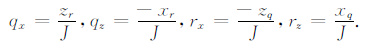
|
(4) |
J是变换的雅克比,它可以表示为J=xqzr-xrzq,详细的推导过程请参见[46].
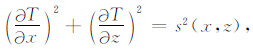
2.2 曲线坐标系中的程函方程笛卡尔坐标系各向同性介质中的程函方程为
|
(5) |
这一方程给出了射线经过慢度为s(x,z)的介质中的点(x,z)时的走时T(x,z).
利用关系式(2a, b),方程(5)可变换为

|
(6) |
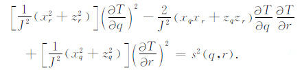
利用方程(4)来替换上式中的度量导数qx,qz,rx,rz,则程函方程(6)可进一步变换为
|
(7) |
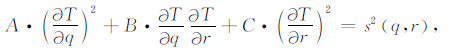
此方程即为曲线坐标系中的程函方程,是Hamilton-Jacobi方程中常见的一种.上述方程可记为下列更为紧凑的形式
|
(8) |
其中,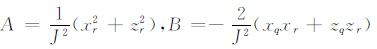
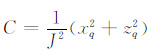
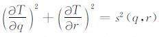
如果不考虑各向异性的程函方程(7)式与各向同性程函方程的差别,则可以把程函方程(8)式离散为下列的形式
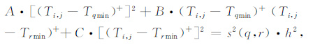
|
(9) |
其中A、B、C的含义与(7)式相同,h为曲线坐标系中的网格间距,Tqmin = min(Ti-1,j,Ti+1,j),Trmin =min(Ti,j-1,Ti,j+1)且
|
(10) |
图 2描述了用快速推进法求解离散的程函方程的详细过程.首先初始化震源点,其走时在后续计算中保持不变.我们把震源点周围的点的走时按从小到大的顺序存在一个数组里,那么它就构成了这一时刻的波前.取出其中的最小值,固定它的值(在后续迭代中保持不变),所有周围未被固定的点的值可按下式进行迭代:

|
(11) |
其中aa=A+B+C,bb=2·A·Tqmin+B·(Tqmin+Trmin)+2·C·Trmin, cc= A·Tqmin2 +B·Tqmin·Trmin +C·Trmin2 -h2 ·s2 .我们把走时为min(Tqmin, Trmin)的点记为(ii,jj),di,j表示点(i,j)到点(ii,jj)的实际距离(笛卡尔坐标系中两点间的距离),则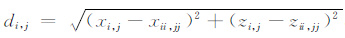

|
图 2 快速推进法更新步骤[19] 网格点可以被分为:活动点、试验点和远点.活动点(黑色)是走时已经知道的点.试验点(灰色)是活动点周围的点,这些点上的走时将被计算.试验点的集合被称作窄带.随着窄带的推进,窄带内的点逐渐被更新为活动点.远点表示走时还未计算的点.当走时传播时,远点逐渐变为试验点.图(a-f)显示了走时传播的顺序:(a),黑色的点表示初始的震源点;(b),计算黑点周围的点的走时,这些点由远点变为试验点;(c),取出试验点中走时最小的点(假设为‘A');(d),计算A 点周围的点的走时,这些点由远点变为试验点;(e),取出试验点中走时最小的点(假设为‘D');(f),计算D 点周围的点的走时,这些点由远点变为试验点.如此循环直至遍布整个计算空间. Fig. 2 Updating procedure for the fast-marching method[19] Grid points are classified as ‘alive' ‘trial' and ‘far'. ‘ Alive' points (in black) are those where the values of 丁 are known. ‘Trial' points (in grey) are those around the curve (of 4 alive' points),at which the propagation is to be computed. The set of trial points is called the narrow band. To compute the propagation, points in the narrow band are updated to ‘alive',while the narrow bandadvances. ‘Far' points (in white) are those at which the propagation has not yet been computed. During the propagation, the farpoints are converted into trial points. Figures (a-f) provide an explanation of this sequence: in (a) ,the black point (alive) representsthe initial point; in (b) thevalue of T is computed in theneighborhoodof theblack point; the points in thi s neighborhood areconverted from far (white) to trial (gray) points; in (c) the trial point with the smallest value of T s chosen (for example ‘A'); in(d) values of T are computed in the neighborhood of point A,converting them from far to trial. In (e) the trial point is chosen that has the smallest value ofT ( for example, ‘ D '); in ( f ) points in the neighborhood of D are converted from far to trial, and theprocedure continues m this manner. |
作为求解Hamilton-Jacobi方程的一种迭代方法,快速扫描法近年来得到了迅速发展.Tsai等[55]将其应用到一类基于均一网格上的Godunov 型Hamiltonians的Hamilton-Jacobi方程的求解当中.Kao等[56]提出了一种基于Lax-Friedrichs数值哈密尔顿的(Gauss-Seidel)G-S扫描型算法.它可以求解任意的静态Hamilton-Jacobi方程,这种方法简单易行、收敛速度快.与基于Godunov数值哈密尔顿的方法不同的是基于Lax-Friedrichs数值哈密尔顿的方法需要加一些边界条件.
2.3.2.1 Lax-Friedrichs哈密尔顿
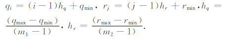
对曲线坐标系中的矩形区域[qmin,qmax]×[rmin,rmax] 进行均匀剖分,网格点记为(qi,rj),i=0,1,…,m1,m1 +1,j= 0,1,…,m2,m2 +1,这里qi= (i-1)hq+qmin, rj= (j-1)hr+rmin, hq=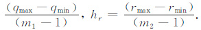
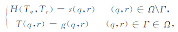
曲线坐标系中的程函方程(8)是一种特殊的静态Hamilton-Jacobi方程,它可以写做如下的形式:
|
(12) |
其中
|
为哈密尔顿算子,A,B,C的意义与前述相同;Ω 为计算区域;Γ 为震源点;s(q,r)是慢度(速度的倒数);g(q,r)为震源点的走时值.
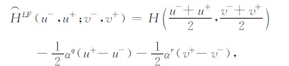
用Lax-Friedrichs格式来离散哈密尔顿算子H(Tq,Tr):
|
(13) |
其中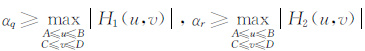
|
(14) |
Tin+1,j表示(i,j)点第n+1次迭代的走时值,这里不写Ti+1,j,Ti-1,j的上标是因为它们的上标与扫描方向有关.对于二维情形,有四个扫描方向:
(1) 从左下角向右上角,即i=1∶m1,j=1∶m2;
(2)从右下角向左上角,即i=m1∶1,j=1∶m2;
(3)从左上角向右下角,即i=1∶m1,j=m2∶1;
(4)从右上角向左下角,即i=m1∶1,j=m2∶1.
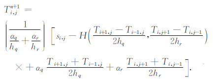
以从左下角向右上角方向扫描,即i= 1∶m1,j=1∶m2 为例,有
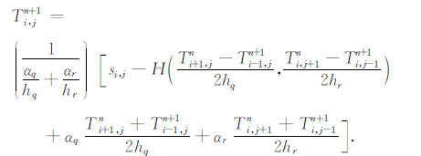
|
(15) |
要指出的是以上的更新公式不涉及任何非线性求逆,因此本文的求解方法很容易实现.
2.3.2.2 计算边界条件由于利用Lax-Friedrichs数值哈密尔顿计算一个网格点的解时需要它周围所有相邻点的信息,因此必须仔细地确定那些超出计算区域的网格点的值.为此,采用Kao等[56]提出的方法处理计算边界,他们结合外推、最大和最小策略计算那些超出计算区域的网格点的值.二维问题的边界条件为
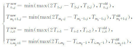
|
(16) |
最后将Gauss-Seidel型Lax-Friedrichs扫描算法作个总结.它主要包含初始化、交替扫描和实施计算边界条件这三个步骤.具体如下:
1.初始化.在边界Γ 上的网格点或邻近的网格点,赋精确值或插值,并且每次迭代过程中这些值固定不变.其它网格点上,赋较大的值M,并且这些值在迭代过程中被更新,这里M应该大于真解的最大值.
2.交替扫描.在第n+1 次迭代时,除了那些赋了精确值或插值的网格点,按照(11)计算Ti,jn+1在所有网格点(qi,rj),1≤i≤m1,1≤j≤m2 的值,并且只有当它小于以前的值Ti,jn时才更新Ti,jn+1.值得注意的是,这个过程需要按交替扫描方向进行,即在二维情形需要四个不同的扫描方向.一般来说,d维情形需要2d次交替扫描.
3.实施计算边界条件.每次扫描之后,按照(16)实施计算边界条件,不同的边界只需作一些细微的修改.
4.收敛准则.如果‖Tn+1-Tn‖L1 ≤δ,算法收敛并终止,这里δ是一个给定的收敛阀值.
3 计算实例为了研究本文给出的两种数值方法求解曲线坐标系程函方程的正确性和适用性,我们首先考虑一个水平地表模型,然后对一组地表地形为余弦函数的起伏地表模型进行计算分析.
为了便于与解析解对比,我们假设模型中介质都是均匀的,速度均为2000m/s.
3.1 水平地表模型模型大小为 [-1km, 1km]2,震源坐标约为(-0.25km, 0.50km).我们把两种数值方法计算的数值解与解析解进行对比,结果见走时等值线图 3,图 4为两种方法计算的结果的绝对误差分布图.由图可知,直接拓展求解各向同性程函方程的快速推进法与用Lax-Friedrichs快速扫描法所求得的数值解都与解析解吻合的较好,且前者的精度更高.这也可以从过炮点且分别与纵轴和横轴平行的两条测线上的走时值中(图 5)观察到.这是因为,对于水平地表的模型,此时各向异性的程函方程(7)就退化为各向同性的程函方程(5),而(16)也就退化为求解各向同性程函方程的迎风差分格式,因此得到更为准确的解;Lax-Friedrichs快速扫描法不是迎风格式的,但是它具有很强的健壮性,对任意形式的Hamiltonians都可以求解,这可以通过后面的实例得到验证.

|
图 3 水平地表模型当震源坐标为(-0.25km, 0.50km)时的初至波走时等值线图 黑色实线表示解析解;红色虚线表示直接拓展求解各向同性程函方程的快速推进法所得的数值解;绿色虚线表示用Lax-Friedrichs快速扫描法求得的数值解,走时等值线的单位为秒. Fig. 3 Traveltime contours (in seconds) for the flat surfacemodel with the source located at (-0.25 km, 0.50 km) The black solid line denotes the analytical solution, while the red and green dashed lines denote numerical solutions obtained by a simple modification of the fatt marching method for the isotropic eikoml equation and Lax-Friedrichs fatt sweeping method. |

|
图 4 直接拓展求解各向同性程函方程的快速推进法(a)和Lax-Friedrichs快速扫描法(b)所得的数值解的绝对误差分布 Fig. 4 Absoiute error maps for the numericai soiutions obtained by a simple modification of the fast marching method forthe isotropic eikonai equation (a) and Lax-Friedrichs fast sweeping method (b),respectively. The units in the error mapsare second (s). |

|
图 5 用两种方法计算的过炮点且分别与纵轴(a)和横轴(b)平行的两条测线上的走时值及其相应的解析解对比. 黑色实线表示解析解;红色虚线表示直接拓展求解各向同性程函方程的快速推进法所得的数值解;绿色虚线表示用Lax-Friedrichs快速扫描法求得的数值解. Fig. 5 Comparisons of travel imes at the two lines which cross the source andparallel z-and x- coordinates, respectively. The black solid line denotes the analytical solution, while the red and green dashed lines denote numerical solutions obtained by a simplemodification of the fast marching method for the isotropic eikonal equation and Lax- Friedrichs fast sweeping method, respectively. |
选取一组起伏地表模型进行研究.模型表面是由一个山丘和两个凹陷组合成的起伏型地表.它的高程可以用下面的余弦函数来表示

|
(17) |
其中,A为余弦函数的振幅,A取值不同表示地表地形起伏的剧烈程度不同,分别取A为0.1、0.2来进行研究.一般的,复杂地表下的走时很难用解析的方法进行刻画,但在地表地形可以用解析式表示的情况下,其解析解还是可以求解的.对于这两个起伏地表的均匀介质模型,计算出其相应的解析解(见附录)并和本文计算的数值解对比来考查本文数值方法求解曲线坐标系程函方程的正确性.
图 6为当A取0.2 时模型的结构化网格剖分图.当A=0.1时,震源坐标分别为(-0.25km, 0.50km),(-0.25km, 0.88km),把两种方法计算的数值解与解析解做一对比,结果见图 7.从图中可以观察到,Lax-Friedrichs快速扫描法计算的结果与解析解吻合的较好,而直接拓展求解各向同性程函方程的快速推进法所得的数值解与解析解出现了较大偏差,这是因为此时曲线坐标系中的程函方程(7)为各向异性的,且随着地表附近贴体网格的扭曲程度逐渐加重方程(7)的各向异性增强[57](可以从曲线坐标系的等值线图 8中观察到),简单的拓展求解各向同性程函方程的快速推进法所得的差分格式(12)并不是方程(7)的正确的迎风格式的离散形式.而Lax-Friedrichs快速扫描法对各向异性的程函方程也是适用的.从地表的走时曲线(图 9)也可以得到类似的结论.

|
图 6 地表地形为z(x)=1.0+0.2cos(1.5πx)km 的模型结构化网格剖分 为清楚起见,网格密度减少为原来的1/8.倒立的黑色三角形表示在起伏的地表上布设的检波器,水平距离从-1到1km Fig. 6 The boundary conforming grids for the modelwhose surface is described by the functionz(x)=1. 0 + 0. 2cos(1.5πx)km For clarity, the grids are displayed with a reducing density factor of 8. The inverted black triangles denote the receivers located at the irregular surface, with horizontal distances between -1 and 1 km. |

|
图 7 振幅为0.1km 的余弦型起伏地表模型震源坐标分别约为(a)(-0.25km, 0.50km),(b)(-0.25km, 0.88km)时的初至波走时等值线图 黑色实线表示解析解;红色虚线表示直接拓展求解各向同性程函方程的快速推进法所得的数值解;绿色虚线表示用Lax-Friedrichs快速扫描法求得的数值解,走时等值线的单位为秒. Fig. 7 Traveltime contours (in seconds) for the model whose surface is a cosine curve-like feature The source is at (a)(-0. 25 km, 0. 50 km) and (b)(-0. 25 km, 0. 88 km),respectively . The black solid line denotes the analytical solution, while the red and green dashed lines denote numerical solutions obtained by a simple moditication of the fast marching method forthe isotropic eikonal equation and Lax-Friedrichs fast sweeping method, respectively. |

|
图 8 振幅为0.1km 的余弦型起伏地表模型震源坐标分别约为(a)(-0.25km, 0.50km),(b)(-0.25km, 0.88km)时在曲线坐标系中的初至波走时等值线图 Fig. 8 Traveltime contours (in seconds) in the curvilinear coordinate for the model whose surface is a cosine curve-like feature |

|
图 9 振幅为0.1(km)的余弦型起伏地表模型地表上走时的数值解与解析解对比 震源坐标分别约为(a)(-0.25km, 0.50km),(b)(-0.25km, 0.88km).黑色实线表示解析解;红色虚线表示直接拓展求解各向同性程函方程的快速推进法所得的数值解;绿色虚线表示用Lax-Friedrichs快速扫描法求得的数值解. Fig. 9 Comparison of travel times of the analytical and numerical solutions at the irregular surface for the model whosetopography amplitude is 0. 1 km with the source located at (a) (— 0.25 km, 0.50 km) and (b) (— 0.25 km, 0.88 km). The black solid line denotes the analytical solution, while the red and green dashed lines denote numerical solutions obtained by a smplemodification of the fast marching method for the isotropic eikonal equation and Lax-Friedrichs fast sweeping method, respectively. |
当A取0.2 时,地表地形起伏更加剧烈,对于地表附近的点,方程(7)的各向异性较A=0.1 时强.此时离散格式(12)已无法求解(根式下出现负数),而用而Lax-Friedrichs快速扫描法求解依然可以得到正确稳定的解,分别见图 10、11.这进一步证实了我们前面的结论.

|
图 10 振幅为0.2(km)的余弦型起伏地表模型当震源分别位于(a)(-0.2km, 1.1km),(b)(-0.2km, -0.1km)时走时等值线图 红线表示解析解,蓝表示数值解(Lax-Friedrich快速扫描法求得的结果),走时等值线的单位为s. Fig. 10 Traveltime contours (in seconds) for the model whose topography amplitude is 0. 2 kmwith the source located at (a) (-0.2 km, 1.0 km) and (b) (-0.2 km, -0.1 km) The red and blue lines denote the analytical and numerical solutions (Computed by the Lax-Friedrichs fast sweeping method) ,respectively. |

|
图 11 振幅为0.2km 的余弦型起伏地表模型地表上走时的数值解(Lax-Friedrich快速扫描法求得的结果)与解析解对比 震源坐标分别为(a)(-0.2km, 1.1km),(b)(-0.2km, -0.1km).黑色虚线和实线分别表示解析解和数值解. Fig. 11 Comparison of travel times of the analytical and numerical (Computed by the Lax-Friedrichs fast sweeping method) solutions at the irregular surface for the model whose topography amplitude is 0. 2 km with the source located at (a) (-0.2 km, 1.1 km),(b) (-0. 2 km, -0. 1 km),respectively. The dotted and solid lines show, respectively, the analytical and numerical solutions. |
为了进一步考查本文的方法,我们选取了一个地表剧烈起伏的模型,Sun等[49]在模拟起伏地表的走时也选用了类似的模型.模型大小为1.6km×1.32km, 地表在1.1~1.32km 之间起伏,表示的地形为两个山丘和两个凹陷的交替组合.用1280×960的网格来离散此模型,剖分的贴体网格见图 12.震源点的坐标为(0.8km, 1.1km),把以震源为圆心半径为0.1km 的区域内的点的初值赋为精确值.图 13为剧烈起伏地表下的Marmousi模型的初至波走时图.由图可见,Lax-Friedrichs快速扫描法对地表地形起伏剧烈,速度纵横向变化剧烈的介质依然具有很好的适用性和稳定性.对于此模型,直接用快速推进法依然无法求解.

|
图 12 剧烈起伏地表模型结构化网格剖分 为清楚起见,网格密度减少为原来的1/8.倒立的黑色三角形表示在起伏的地表上布设的检波器,水平距离从0到1.6km. Fig. 12 The boundary conforming grids n the severe undulated surface model For clarity, the grids are displayed with a reducing density factor of 8. The inverted black triangles denote the receivers located at the irregular surface, with horizontal distances between 0 and 1. 6 km. |

|
图 13 剧烈起伏地表下的Marmousi模型中初至波走时等值线.震源坐标为(0.8km, 1.1km). Fig. 13 Traveltime contours (in seconds) superimposed on the revised Marmousi model, the source is located at (0. 8 km, 1. 1 km). |
复杂地表条件下的地震波走时计算对于实现复杂地表条件下的静校正、偏移成像、走时反演、层析成像、地震定位等具有重要意义.借助于贴体网格,把笛卡尔坐标系中的程函方程变换到曲线坐标系中,然后,尝试采用直接拓展各向同性程函方程的快速推进法和Lax-Friedrichs快速扫描算法求解曲线坐标系的程函方程.数值实例表明,此时在曲线坐标系中程函方程已变为各向异性的程函方程,因此通过直接拓展各向同性程函方程的快速推进法来求解该方程是错误的,而用Lax-Friedrichs快速扫描法求解总能得到稳定正确的解,这对于起伏地表的走时计算具有重要意义.
附录:复杂地表下均匀介质模型中的精确走时计算策略一般的,复杂地表下的走时很难用解析的方法进行刻画,但在地表地形可以用解析式表示的情况下,其解析解还是可以求解的.在此,我们就来探讨本文模型的解析解的求解.
以地表地形为振幅为0.2km 的余弦曲线模型为例来介绍其精确走时的求解.首先,讨论震源在点(-0.2km, 1.1km)的情形,对于其它情形后续在讨论.求解的难点是如何确定从震源到区域内其它点的射线的最短路径.根据从震源‘S'到模型内其它点的射线路径的形态,求解区域可以被剖分为三部分,如图 A1a显示的两个灰色区域和白色区域的部分.对于白色区域内的点,从震源到该点的最短射线路径均为直线,因此其走时很容易求得.对于两个灰色区域,我们以左上角的灰色区域为例来介绍,右上角的区域可类似计算.对于灰色区域内的一点B(弧$\overset\frown{DM}$下方,线段DE上方),过该点做一条直线与$\overset\frown{DM}$相切,切点为C(在$\overset\frown{DC}$上),那么此时从震源S到点B的最短射线路径为SD+$\overset\frown{DC}$+CB(易被证明,在此从略),向量SD和CB的长度可以通过两点间距离公式求得,而$\overset\frown{DC}$的长度可以通过弧长公式计算得出.进而可以求出其相应的走时.同理,可以计算出此区域内其它点的走时.

|
图 图A1 本文中的起伏地表模型走时计算策略 S表示震源,SE、SF分别切余弦曲线于点D、G;A表示地表曲线上一点,B表示曲线下一点;CB切余弦曲线于点C;曲线交左右边界分别于点M、N. Fig. 图A1 The strategy for computing analytical solutions of travel times for the irregular surface models of this paper S denotes the source for this model; SE and SF are two vectors which are tangent to the cosine curve (irregular surface) at points D and G,respectively; A denotes a point on the surface curve, while B denotes a point beneath the surface; CB is tangent to the cosine curve at point C; the cosine curve intersects the lett and right boundaries at points M and N,respectively. |
由于弧$\overset\frown{MD}$和$\overset\frown{NG}$为严格的凹曲线,因此对于这两段弧上的点,最短射线路径只包括两部分,即一根线段和一段圆弧.以点‘A'为例,从震源点‘S'到该点的最短射线路径为SD+$\overset\frown{DA}$,它的长度可以通过前面介绍的方法求得.
当震源位于点(-0.2km, -0.1km)(图 A1(b))上时,只有右上角一小部分区域内的点需要按照上述的方法特别处理.
综上所述,我们就可以求得该模型中的初至波精确走时.对于其它模型的情况可以类似求解,这里从略.
致谢本研究工作得到了中国科学院地质与地球物理研究所张中杰研究员的悉心指导和帮助.三位审稿专家对本研究工作提供了许多建设性的意见.笔者在此表示衷心的感谢.
| [1] | Aki K, Richards P G. Quantitative seismology. 2002: Univ Science Books. |
| [2] | Hole J. Nonlinear high-resolution three-dimensional seismic travel time tomography. Journal of Geophysical Research , 1992, 97(B5): 6553-6562. |
| [3] | Chen Y, Badal J, Hu J. Love and Rayleigh wave tomography of the Qinghai-Tibet Plateau and surrounding areas. Pure and Applied Geophysics , 2010, 167(10): 1-33. |
| [4] | Zelt C, Smith R. Seismic traveltime inversion for 2-D crustal velocity structure. Geophysical Journal International , 1992, 108(1): 16-34. DOI:10.1111/gji.1992.108.issue-1 |
| [5] | Zhang Z J, Wang G J, Teng J W, et al. CDP mapping to obtain the fine structure of the crust and upper mantle from seismic sounding data: an example for the southeastern China. Physics of the Earth and Planetary Interiors , 2000, 122(1-2): 133-146. DOI:10.1016/S0031-9201(00)00191-6 |
| [6] | 张中杰, 秦义龙, 陈赟, 等. 由宽角反射地震资料重建壳幔反射结构的相似性剖面. 地球物理学报 , 2004, 47(3): 469–474. Zhang Z J, Qin Y L, Chen Y, et al. Reconstruction of the semblance section for the crust and mantle reflection structure by wide-angle reflection seismic data. Chinese J. Geophys. (in Chinese) , 2004, 47(3): 469-474. |
| [7] | 朱金明, 王丽燕. 地震波走时的有限差分法计算. 地球物理学报 , 1992, 35(1): 86–92. Zhu J M, Wang L Y. Finite difference calculation of seismic travel times. Chinese J. Geophys. (in Chinese) , 1992, 35(1): 86-92. |
| [8] | Cerveny V, Molotkov I A, and Psencik I. Ray methods in seismology. 1977, Univ. of Karlova Press. |
| [9] | Zhang Z, Badal J, Li Y, et al. Crust-upper mantle seismic velocity structure across Southeastern China. Tectonophysics , 2005, 395(1-2): 137-157. DOI:10.1016/j.tecto.2004.08.008 |
| [10] | Zhang Z, Li Y, Lu D, et al. Velocity and anisotropy structure of the crust in the Dabieshan orogenic belt from wide-angle seismic data. Physics of the Earth and Planetary Interiors , 2000, 122(1-2): 115-131. |
| [11] | Zhang Z, Wang Y, Chen Y, et al. Crustal structure across Longmenshan fault belt from passive source seismic profiling. Geophys. Res. Lett , 2009, 36. |
| [12] | Xu T, Xu G, Gao E, et al. Block modeling and segmentally iterative ray tracing in complex 3D media. Geophysics , 2006, 71: T41-T51. DOI:10.1190/1.2192948 |
| [13] | Xu T, Zhang Z, Gao E, et al. Segmentally Iterative Ray Tracing in Complex 2D and 3D Heterogeneous Block Models. Bulletin of the Seismological Society of America , 100(2): 841-850. DOI:10.1785/0120090155 |
| [14] | Vidale J E. Finite-difference calculation of travel times. Bulletin of the Seismological Society of America , 1988, 78(6): 2062-2076. |
| [15] | Vidale J E. Finite-difference calculation of traveltimes in three dimensions. Geophysics , 1990, 55(5): 521-526. |
| [16] | Qin F, Luo Y, Olsen K B, et al. Finite-difference solution of the eikonal equation along expanding wavefronts. Geophysics , 1992, 57: 478-487. DOI:10.1190/1.1443263 |
| [17] | Van Trier J, Symes W W. Upwind finite-difference calculation of traveltimes. Geophysics , 1991, 56(6): 812-821. |
| [18] | Sethian J. Evolution, implementation, and application of level set and fast marching methods for advancing fronts. Journal of Computational Physics , 2001, 169(2): 503-555. DOI:10.1006/jcph.2000.6657 |
| [19] | Sethian J A. Fast marching methods. SIAM review , 1999, 41(2): 199-235. |
| [20] | Sethian J A, Popovici A M. Three dimensional traveltimes computation using the Fast Marching Method. Geophysics , 1999, 64(2): 516-523. DOI:10.1190/1.1444558 |
| [21] | Sethian J A. A fast marching level set method for monotonically advancing fronts. Proceedings of the National Academy of Sciences of the United States of America , 1996, 93(4): 1591-1595. |
| [22] | Alkhalifah, T. & Fomel, S .. Implementing the fast marching eikonal solver: spherical versus Cartesian coordinates. Geophys. Prospect. , 2001, 49: 165-178. DOI:10.1046/j.1365-2478.2001.00245.x |
| [23] | Fomel S. A variational formulation of the fast marching eikonal solver. SEP-95: Stanford Exploration Project, 1997 : 127 -147. |
| [24] | Kim S. 3-D eikonal solvers: First-arrival traveltimes. Geophysics , 2002, 67(4): 1225-1231. |
| [25] | Rawlinson N, Sambridge M. Wave front evolution in strongly heterogeneous layered media using the fast marching method. Geophysical Journal International , 2004, 156(3): 631-647. DOI:10.1111/gji.2004.156.issue-3 |
| [26] | Rawlinson N, Sambridge M. Multiple reflection and transmission phases in complex layered media using a multistage fast marching method. Geophysics , 2004, 69(5): 1338. |
| [27] | Rawlinson N, Sambridge M. The fast marching method: an effective tool for tomographic imaging and tracking multiple phases in complex layered media. Exploration Geophysics , 2005, 36(4): 341-350. |
| [28] | 孙章庆, 孙建国, 韩复兴. 复杂地表条件下基于线性插值和窄带技术的地震波走时计算. 地球物理学报 , 2009, 52(11): 2846–2853. Sun Z Q, Sun J G, Han F X. Travehimes computation using linear interpoiation and narrow band technique under complex topographical conditions. Chinese J.Geophys. (in Chinese) , 2009, 52(11): 2846-2853. |
| [29] | De Kool M, Rawlinson N, Sambridge M. A practical grid-based method for tracking multiple refraction and reflection phases in three-dimensional heterogeneous media. Geophysical Journal International , 2006, 167(1): 253-270. DOI:10.1111/gji.2006.167.issue-1 |
| [30] | Zhao H. A fast sweeping method for eikonal equations. Mathematics of Computation , 2005, 74(250): 603-628. |
| [31] | Zhang Y T, Zhao H K, Qian J. High order fast sweeping methods for static Hamilton-Jacobi equations. Journal of Scientific Computing , 2006, 29(1): 25-56. |
| [32] | 兰海强,张智,徐涛等.地震波走时场模拟的快速推进法和快速扫描法比较研究.地球物理学进展,2012,已接受. Lan H Q, Zhang Z, Xu T, et. al. A comparative study on the fast marching and fast sweeping methods in the calculation of first-arrival traveltime field. Progress in Geophys.,2012, accepted. |
| [33] | Zhang Z J, Yang L Q, Teng J W, Badal J. An overview of the earth crust under China. Earth-Science Reviews , 104(1-3): 143-166. DOI:10.1016/j.earscirev.2010.10.003,2011 |
| [34] | Lan H, Zhang Z. Three-dimensional wave-field simulation in heterogeneous transversely isotropic medium with irregular free surface. Bulletin of the Seismological Society of America , 2011, 101(3): 1354-1370. |
| [35] | 阎世信, 刘怀山, 姚雪根. 山地地球物理勘探技术. 北京: 石油工业出版社, 2000 . Yan S X, Liu H S, Yao X G. Geophysical Exploration Technology in the Mountainous Area (in Chinese). Beijing: Petroleum Industry Press, 2000 . |
| [36] | Kao C Y, Osher S, Qian J. Legendre-transform-based fast sweeping methods for static Hamilton-Jacobi equations on triangulated meshes. Journal of Computational Physics , 2008, 227(24): 10209-10225. DOI:10.1016/j.jcp.2008.08.016 |
| [37] | Kimmel R, Sethian J A. Computing geodesic paths on manifolds. Proceedings of the National Academy of Sciences of the United States of America , 1998, 95(15): 8431-7435. DOI:10.1073/pnas.95.15.8431 |
| [38] | Lelièvre P G, Farquharson C G, Hurich C A. Computing first-arrival seismic traveltimes on unstructured 3-D tetrahedral grids using the Fast Marching Method. Geophysical Journal International , 184(2): 885-896. DOI:10.1111/gji.2011.184.issue-2 |
| [39] | Qian J, Zhang Y T, Zhao H K. A fast sweeping method for static convex Hamilton-Jacobi equations. Journal of Scientific Computing , 2007, 31(1): 237-271. |
| [40] | Qian J, Zhang Y T, Zhao H K. Fast sweeping methods for Eikonal equations on triangular meshes. SIAM Journal on Numerical Analysis , 2008, 45(1): 83-107. |
| [41] | Sethian J A, Vladimirsky A. Fast methods for the Eikonal and related Hamilton-Jacobi equations on unstructured meshes. Proceedings of the National Academy of Sciences of the United States of America , 2000, 97(11): 5699. DOI:10.1073/pnas.090060097 |
| [42] | Appelo D, Petersson N. A stable finite difference method for the elastic wave equation on complex geometries with free surfaces. Communications in Computational Physics , 2009, 5(1): 84-107. |
| [43] | 孙章庆, 孙建国, 张东良. 二维起伏地表条件下坐标变换法直流电场数值模拟. 吉林大学学报: 地球科学版 , 2009, 39(3): 528–534. Sun Z Q, Sun J G, Zhang D L. 2D DC electric field numerical modeling including surface topography using coordinate transformation method. Journal of Jilin University: Earth Science Edition (in Chinese) , 2009, 39(3): 528-534. |
| [44] | Lan H, Zhang Z. 2D finite-difference seismic modeling of an open fluid-filled fracture with irregular free surface, in review |
| [45] | Tessmer E, Kosloff D. 3-D elastic modeling with surface topography by a Chebychev spectral method. Geophysics , 1994, 59: 464. DOI:10.1190/1.1443608 |
| [46] | 兰海强, 刘佳, 白志明. VTI介质起伏地表地震波场模拟. 地球物理学报 , 2011, 54(8): 2072–2084. Lan H Q, Liu J, Bai Z M. Wave-field simulation in VTI media with irregular free surface. Chinese J.Geophys. (in Chinese) , 2011, 54(8): 2072-2084. |
| [47] | 孙建国. 复杂地表条件下地球物理场数值模拟方法评述. 世界地质 , 2007, 26(003): 345–362. Sun J G. Methods for numerical modeling of geophysical fields under complex topographicaI conditions:a critical review. Global Geology (in Chinese) , 2007, 26(003): 345-362. |
| [48] | Lan H, Zhang Z. Comparative study of the free-surface boundary condition in two-dimensional finite-difference elastic wave field simulation. Journal of Geophysics and Engineering , 2011, 8: 275-286. DOI:10.1088/1742-2132/8/2/012 |
| [49] | Sun J, Sun Z, Han F. A finite difference scheme for solving the eikonal equation including surface topography. Geophysics , 2011, 76(4): T53-T63. |
| [50] | Zhang Z J, Teng J W, Wan Z C. Establishment of parametric equations of seismic-wavefronts in 2-D anisotropic media. Chinese Science Bulletin , 1994, 39(22): 1890-1894. |
| [51] | Hvid S L. Three dimensional algebraic grid generation , Technical University of Denmark,1994. |
| [52] | Thompson J, Warsi Z, Mastin C. Numerical grid generation: foundations and applications. 1985: North-holland Amsterdam. |
| [53] | Hestholm S, Ruud B. 3-D finite-difference elastic wave modeling including surface topography. Geophysics , 1998, 63: 613-622. |
| [54] | Tessmer E, Kosloff D, Behle A. Elastic wave propagation simulation in the presence of surface topography. Geophys. J. Int , 1992, 108(2): 621-632. DOI:10.1111/gji.1992.108.issue-2 |
| [55] | Tsai Y H R, Cheng L T, Osher S, et al. Fast sweeping algorithms for a class of Hamilton-Jacobi equations. SIAM Journal on Numerical Analysis , 2004: 673-694. |
| [56] | Kao C Y, Osher S, Qian J. Lax-Friedrichs sweeping scheme for static Hamilton-Jacobi equations. Journal of Computational Physics , 2004, 196(1): 367-391. DOI:10.1016/j.jcp.2003.11.007 |
| [57] | 兰海强,徐涛,白志明.贴体网格各向异性对坐标变换法求解起伏地表下地震初至波走时的影响研究.地球物理学报,已接受. Lan H Q, Xu T, Bai Z M. Study of the effects due to the anisotropic stretching of the surface-fitting grid on the traveltime computation for irregular surface by the coordinate transforming method. Chinese J.Geophys.,in press. |