 2010, Vol. 53


可控源电磁法(CSEM)广泛应用于金属矿、石油天然气、地下水、地热资源勘探及各种工程勘察领域[1~5].目前, 可控源电磁法在数值模拟、反演解释方面的研究还多限于二维, 甚至一维解释[6~13].随着地质勘探目标越来越复杂、要求越来越高, 可控源电磁法不可避免地要发展三维正、反演方法.现阶段三维地电模型的电磁响应正演计算尤为重要, 尤其是三维反演解释的基础.
地球电磁三维正演模拟方面国内外学者均做了不少工作, 其中以大地电磁测深的有限差分法和积分方程法的电磁三维模拟居多[14~22], 而针对可控源电磁三维有限元模拟的工作还很少[23, 24], 主要问题是电磁场的电场在界面上的法向分量不连续, 不符合节点有限元中函数在求解域内连续的要求.早期的有限元模拟通常忽略这一问题, 导致可能获得不正确的解[23].如果不直接求解电磁场, 而求解电磁场的位势, 则出现伪解现象, 同时还存在数值不稳定性[25~29].本文研究水平电偶极子源在三维介质中的电磁场分布, 采用磁场矢量位和电场标量位作为计算对象, 求得各节点上的位势后用差商求得电磁场的值.由于电磁场的位势满足的是类似Helmoltz类型的方程, 采用有限单元法求解Helmholtz方程必然会引起数值不稳定, 我们引入罚项及稳定化有限单元方法, 保证计算过程稳定并获得可靠的电磁场的解.
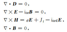
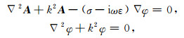
2 数学模型设时间因子的形式为e-iωt, 则除源以外的导电介质中, 频率域的Maxwell方程组形式如下:
|
(1) |
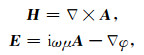
其中D是电位移矢量, E为电场强度矢量, H、B分别是磁场强度及磁感应强度矢量, ε为介电常数, Jf是激励源, 即水平电偶极子.在导电介质中, 一般假设介质的导磁率为真空导电磁率, 介质的介电常数为真空介电常数.由于电场在界面上的法向分量不连续, 不能使用节点有限元法直接求解方程组(1).引进磁矢量势A和电场标量势φ, 磁场和电场表示成如下形式[30]:
|
(2) |
显然, 由磁场的连续性可以得到A的连续性.在电性界面上, 电场的切向分量是连续的, 结合A的连续性, 可以得到A在界面上的法向分量是连续的, 由式(2)的第二式, 可以得到n× (Δ φ1 -Δ φ2)=0, n是界面的单位法向量, 故可以得到φ是连续的, 即

|
对于取φ恒为零的特例, 则E=iωμA, 由于在界面上, 电场E法向分量是不连续的, 似乎矢势A也应不连续.其实, 由方程(1)的第一式可以得到▽·A=0, 在方程(1)的第三式取散度, 得到Δ·(σA)=0, 即A· Δ σ=0, 在电性界面上, 电导率的梯度方向是和界面的法向方向一致的, 故A在界面上法向分量为零, 上面的不连续性是不存在的, 而且, 为了保证在界面上电场的法向分量不为零, 不能取φ恒为零.所以, A和φ在全空间是连续的.
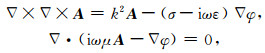
将(2)式代入方程(1)的第一式和三式, 则:
|
(3) |
其中k2=ω2εμ +iωμσ, 激励源Jf将在边界条件中单独处理, 因而上式未做考虑.
在使用势求电磁场时, 一般首先求矢量势, 然后由规范条件求出标量势.本文使用的是Lorentz规范, 人工边界上的值就是使用Lorentz规范得到的.但是, 有限元模拟中A的插值函数是一阶近似的线性插值, 若由Lorentz规范条件▽·A+(σ-iωε)φ=0从A求φ, 则φ就是零级近似了.因此, 为了保证A和φ的数值解有相同的精度, 必须同时求解A和φ.
在数值求解▽×▽×A-k2A=0的方程时, 会产生伪解, 以下给出二维情况下的分析.设A=
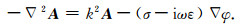
本文中, 采用节点有限元法离散方程(3)的第一式时, 由于▽ × ▽ ×A会产生不对称的有限单元矩阵, 引起数值不稳定, 详细的分析请参考文献[26~29].为了排除伪解和保证数值稳定, 在方程组(3)的第一式左端加上一罚项-p ▽▽·A, 即:
▽ × ▽ ×A-p ▽▽·A=k2A-(σ-iωε) Δ φ.取p=1, 由▽ × ▽×A=▽▽·A-Δ2A, 得
|
对于方程(3)的第二式, 其显然不是类似于Helmholtz型的方程, 使用Lorentz规范将其化为φ的Helmholtz方程, 即:
|
(4) |
方程组(4)为Helmholtz类型的方程.
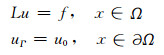
3 边界条件由于研究区域远离源, 因而把源纳入计算区域将大大增加网格剖分单元, 从而计算量也大大增加.本文用计算区域人工边界Г的第一类边界条件来表达源Jf的作用, 即:

|
(5) |
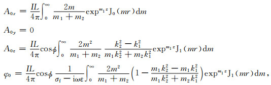
其中A0, φ0为源在均匀半空间的解.对于偶极矩为IL的水平电偶极子, 在空气中的解为[30]:
|
(6) |
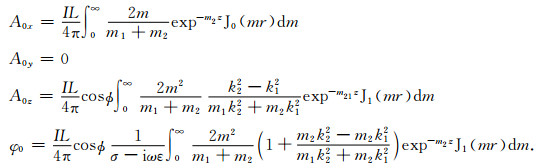
在地下介质中的解导出如下:
|
(7) |
式中σf为空气层的电导率, σ为下半介质空间的电导率, 
采用滤波算法计算上面各式的值[31].
4 稳定化有限单元法计算 4.1 稳定化有限单元法Helmholtz方程描述的是时谐波的方程, 其随着波数的增大, Galerkin有限元法解的精度下降.为了克服这个困难, 诸多学者发展了多种有限单元法, 如广义有限元法或者说叫稳定化有限单元法[32~38].一般的满足第一类边界的Helmholtz方程为:
|
其中,
|
标准的Galerkin有限元法如下:
|
其中(·, ·)表示L2(Ω)的标量积.
广义Galerkin有限元的形式如下:
|
其中算子L*是算子L的伴算子, τ是稳定化常数; K表示对单元求和.详细的分析请参考文献[32~38].方程组(4)第一个方程对应的L(A, φ)=▽2A+k2A-(σ-iωε)▽φ, 取L*u=▽2u+k2u, 且插值函数是线性函数, 则▽2u1=0, 把上面的公式用于方程组(4), 得到
|
(8) |
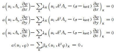
其中a(u, A, φ)=(u, ▽2A)+(u, k2A)-(u, (σ-iωε)φ) a(u, φ)=(u, ▽2 φ)+ (u, k2 φ),
(·, ·)K的积分区域是单元K, λK和βK是与网格、频率相关的常数, 一般来说, 对所有的单元, 取λK相等, βK也取相等, 但λK和βK不相等, 理论上没有很好的方法计算它们, 本文通过试验来确定.
4.2 方程的离散与求解使用长方体等参单元e离散化方程(8)式, 其八个顶点上的场值为未知数, 将所有节点上的场值进行统一编号, 并结合第一类边界条件, 则可以得到如下线性方程组:
|
(9) |
其中,

|
K是刚度矩阵, b是与人工边界有关的项.详细的分析参考文献[39, 40].
方程(9)是一个大型复系数线性方程组, 使用双共轭梯度稳定化方法(BiCGstab)[41]解, 获得u=(Ax1, Ay1, Az1, φ1, …, Axn, Ayn, Azn, φn), 由下式差分形式求得任意方向的电场分量:

|
(10) |
取空气的电导率为106 Ωm, 均匀半空间的电阻率为100Ωm, 计算区域大小为: 4000m×2880m× 1880m, 划分为65×54×32个单元, 勘探区域为2000m×1650 m, 线距为50 m, 点距为40 m, 具体参数见图 1.该均匀半空间模型存在解析解, 其有限元三维数值计算值与解析解进行比较的结果见图 2, 计算误差的公式为:
|
(11) |

|
图 1 模型示意图 实线矩形表示计算区域即人工边界的位置,虚线矩形表示勘探区域. Fig. 1 Schematic drawing of model Solid llne square denotes computation domain i. e. the artificial boundary, dot llne square denotes area for exploration. |
其中f c i是点i处场值的数值计算结果, FA i是点i处场值的解析解.图 2表明, 有限元三维数值计算结果在很宽的频率范围(0.1~1000 Hz)均非常稳定, 计算误差基本小于2%.

|
图 2 不同频率上电场值的数值计算结果相对误差 Fig. 2 Relative errors of numerical solutions of electrical field at differential frequencies |
图 3是均匀半空间中存在一个低阻异常体的模型示意图.均匀半空间电阻率为100Ωm, 异常体大小为200m×240m×260m, 埋深为160m, 电阻率为10Ωm, 具体参数见图 3.三维有限元的计算结果见图 4, 给出了1000Hz、250Hz、0.1Hz的电场Ex的实部、虚部以及视电阻率平面等值线图.其中, 视电阻率沿x方向观测, 符合赤道偶极装置条件, 其远区视电阻率表达式为

|

|
图 3 个异常体三维模型示意图 黑色区域表示异常体在地面上的投影, 电阻率为1 0 Ωm. Fig. 3 Schematic drawing of model with a single anomaly Black area denotes the conductive media with resistivity of 10 Ωm. |

|
图 4 不同频率电场Ex(V /m)和视电阻率(Ωm)等值线图 (a 1, a 2, a 3)为1 0 0 0Hz的电场Ex实部、虚部以及视电阻率; (b 1, b 2, b 3)为2 5 0Hz的电场Ex的实部、虚部以及视电阻率; (c 1, c 2, c 3)为0. 1Hz的电场Ex的实部、虚部以及视电阻率. Fig. 4 Contour maps of electrical field Ex and apparent resistivity at differential frequencies (a1, a2) is the real and imaginary part of Ex at 1000 Hz and (a3) denotes its apparent resistivity; (b1, b2) is the real and imaginary part of Ex at 250 Hz and (b3) denotes ts apparent resisitivity; (b1, c2) is the real and imaginary part of Ex at 0. 1 Hz and (c3) denotes its apparent resistivity. |
由于三维可控源的电磁响应分布非常复杂, 又没有解析解可比较, 因此利用电场的实部、虚部等值线分布难于说明三维有限元计算结果的可靠性.但视电阻率等值线图很好地显示了低阻异常体的位置; 而且, 频率越高, 电磁响应对低阻异常体的灵敏度越高, 视电阻率相对异常也越大, 1000 Hz的视电阻率等值线图上异常值最低达76Ωm (相对于100Ωm的均匀半空间), 而250 Hz的视电阻率等值线图上异常值仅低至92Ωm.可见, 随着频率的降低, 趋肤深度增大, 电磁波对地下异常体的灵敏度(分辨率)下降, 符合电磁波在地下介质的传播理论.这些结果均表明本文的电磁三维有限元计算结果是正确的.
5.3 两个异常体三维模型图 5是高阻和低阻两个异常体并存的三维模型示意图.均匀半空间电阻率为100Ωm, 异常体大小均为200m×240m×260m, 埋深也均为160m, 两个异常体间的水平距离为400 m, 电阻率分别为10Ωm和1000Ωm.具体参数见图 5.该模型的三维有限元的计算结果见图 6, 同样视电阻率等值线图很好地显示了低阻异常体的位置, 但对高阻体的分辨很低, 几乎没有显示, 这正是电磁感应类方法的明显特点.因为在导电介质中, 异常体主要是通过产生的感应电流显示其存在的, 异常体电阻率越小, 产生的感应电流越强.因此电磁法对良导体有很好的分辩, 相反, 对高阻体的分辨就很弱.

|
图 5 高阻和低阻两个异常体并存的三维模型示意图黑色区域对应的异常体电阻率为1 0Ωm, 灰色区域对应的异常体的电阻率为1 0 0 0Ωm, 均匀半空间电阻率为1 0 0Ωm. Fig. 5 Schematic drawing of 3D model with two anomalies in homogeneous half space of 100 Ωm Black area denotes the conductive media with resistivity of 10 Ωm, grey area denotes the resistive media of 1000 Ωm. |

|
图 6 高阻和低阻三维模型不同频率电场Ex(V /m)和视电阻率(Ωm)等值线图. (a1, a2, a3)为1000Hz的电场Ex实部、虚部以及视电阻率; (b1, b2, b3)为250Hz的电场Ex的实部、虚部以及视电阻率; (c1, c2, c3)为0.1Hz的电场Ex的实部、虚部以及视电阻率 Fig. 6 Contour maps of electrical field Ex and apparent resistivity at differential frequencies for 3D model with two anomalies (a1, a2) is the real and imaginary part of Ex at 1000 Hz and (a3) denotes its apparent resisitivity; (b1, b2) is the real and imaginary part of Ex at 250 Hz and (b3) denotes its apparent resisitivity; (c1, c2) is the real and imaginary part of Ex at 0.1 Hz and (c3) denotes its apparent resisitivity. |
另一方面, 对比图 3的单个低阻异常体模型, 图 5的模型只是低阻异常体位置有变化并加上一高阻异常体.而相比图 4的单个低阻异常体的计算结果, 图 6的计算结果除低阻异常体位置有变化外, 与图 4非常类似.这说明两点, 其一, 电磁法对高阻体的分辨的确很弱; 其二, 本文的三维有限元计算对复杂模型的数值模拟结果也是稳定、可靠的.
图 7是该模型在y=17220m处的频率测深剖面图, 计算频点为1024、512、256、128、64、32Hz, 横轴x表示测线方向, 纵轴表示对应频率电磁波在均匀半空间中的趋肤深度d=503 

|
图 7 频率测深剖面等值线图 (a)为电场实部;(b)为电场的虚部;(c)为视电阻率. Fig. 7 Contour maps of frequency sounding cross-section. (a) The real part of Ex; (b) The imaginary part of Ex; (c) Apparent resistivity. |
本文采用Galerkin有限元法求解电磁场的磁矢量势和电标势的耦合方程, 同时为克服解Maxwell方程组易出现的伪解及数值稳定性问题, 引入了罚项和稳定化有限单元方法.均匀半空间下的模拟结果表明, 解的相对误差基本小于2%;复杂三维模型的有限元数值模拟也获得稳定、可靠的解, 其远区视电阻率分布显示电磁法对良导体有很好的分辩, 为三维可控源电磁反演奠定了基础.
| [1] | 于昌明. CSAMT法在寻找隐伏金矿中的应用. 地球物理学报 , 1998, 41(1): 133–138. Yu C M. The application of CSAM T method in looking for hidden gold mine. Chinese J. Geophys. (in Chinese) , 1998, 41(1): 133-138. |
| [2] | 吴璐苹, 石昆法, 李荫槐, 等. 可控源音频大地电磁法在地下水勘查中的应用研究. 地球物理学报 , 1996, 39(5): 712–7l. Wu L P, Shi K F, Li Y H, et al. Applied study of CSAMT method on groundwater exploration. Chinese J. Geophys. (in Chinese) , 1996, 39(5): 712-7l. |
| [3] | Constable S, Srnka L J. An induction to marine controlled source electromagnetic methods for hydrocarbon exploration. Geophysics , 2007, 72(2): WA3-WA12. DOI:10.1190/1.2432483 |
| [4] | 周厚芳, 刘闯, 石昆法. 地热资源探测方法研究进展. 地球物理学进展 , 2003, 18(4): 656–661. Zhou H F, Liu C Shi K F. A Review of study on geothermal resources exploration. Progress in Geophysics (in Chinese) , 2003, 18(4): 656-661. |
| [5] | 底青云, 伍法权, 王光杰, 等. 地球物理综合勘探技术在南水北调西线工程深埋长隧洞勘察中的应用. 岩石力学与工程学报 , 2005, 24(20): 3631–3638. Di Q Y, Wu F Q, Wang G J, et al. Geophysical exploration over long deep tunnel for west route of South-to-North water transfer project. Chinese Journal of Rock Mechanics and Engineering (in Chinese) , 2005, 24(20): 3631-3638. |
| [6] | 阎述, 陈明生. 线源频率电磁测深二维正演(一). 煤田与地质勘探 , 1999, 27(5): 60–62. Yan S, Cheng M S. Line source frequency electromagnetic sounding two dimensional forward modeling I. Coal Geology & Exploration (in Chinese) , 1999, 27(5): 60-62. |
| [7] | 阎述, 陈明生. 线源频率电磁测深二维正演(二). 煤田与地质勘探 , 1999, 27(6): 56–59. Yan S, Chen M S. Line source frequency electromagnetic sounding two dimensional forward modeling II. Coal Geology and Exploration (in Chinese) , 1999, 27(6): 56-59. |
| [8] | 陈小斌, 胡文宝. 有限元直接迭代算法及其在线源频率域电磁响应计算中的应用. 地球物理学报 , 2002, 45(1): 119–130. Chen X B, Hu W B. Direct Iterative Finite Element algorithm (DIFE) algorithm and its application to electromagnetic response modeling of the line current source. Chinese J. Geophys. (in Chinese) , 2002, 45(1): 119-130. |
| [9] | 底青云, MartynUnsworth, 王妙月. 有限元法2.5维CSAMT数值模拟. 地球物理学进展 , 2004, 19(2): 317–24. Di Q Y, Unsworth M, Wang M Y. 2.5D CSAM T modeling with finite element method. Progress in Geophysics (in Chinese) , 2004, 19(2): 317-24. |
| [10] | Yuji Mitsuhata. 2-D electromagnetic modeling by finite-element method with a dipole source and topography. Geophysics , 2000, 65(2): 465-475. DOI:10.1190/1.1444740 |
| [11] | Yuji Mitsuhata, Toshihiro Uchida, Hiroshi Amano. 2.5D inversion of frequency domain electromagnetic data generated by a grounded-wire source. Geophysics , 2002, 67(6): 1753-1768. DOI:10.1190/1.1527076 |
| [12] | Abubakar A, Habashy T M, et al. 2.5D forward and inverse modeling for interpreting low frequency electromagnetic measurements. Geophysics , 2008, 73(4): F165-F177. DOI:10.1190/1.2937466 |
| [13] | Li Y, Key K. 2D marine controlled-source electromagnetic modeling:Part 1-An adaptive finite-element algorithm. Geophysics , 2007, 72: WA51. DOI:10.1190/1.2432262 |
| [14] | Zhdanov M S, Wannamaker P E. Three dimensional electromagnetics-Proceedings of the second international symposium. Elsevier , 2002. |
| [15] | Mackie R L, Madden T R, Wannamaker P. 3-D magnetotelluric modeling using difference equations theory and comparisons to integral equation solutions. Geophysics , 1993, 58: 215-226. DOI:10.1190/1.1443407 |
| [16] | Newman G A, Alumbaugh D L. Frequency-domain modeling of airborne electromagnetic responses using staggered finite differences. Geophys.Prosp. , 1995, 43: 1021-1042. DOI:10.1111/gpr.1995.43.issue-8 |
| [17] | Smith J T. Conservative modeling of 3 D electromagnetic fields, Part I, Properties and error analysis. Geophysics , 1996, 61: 1308-1318. DOI:10.1190/1.1444054 |
| [18] | Smith J T. Conservative modeling of 3 D electromagnetic fields, Part II, Biconjugate gradient solution and an accelerator. Geophysics , 1996, 61: 1319-1324. DOI:10.1190/1.1444055 |
| [19] | 谭捍东, 余钦范, BookerJ, 等. 大地电磁三维快速松弛反演. 地球物理学报 , 2003, 46(6): 850–855. Tan H D, Yu Q F, Booker J, et al. Three-dimensional rapid relaxation inversion for the magnetotelluric method. Chinese J.Geophys. (in Chinese) , 2003, 46(6): 850-855. |
| [20] | Wannamaker P E. Advances in three-dimensional magnetotelluric modeling using integral equations. Geophysics , 1991, 56: 1716-1728. DOI:10.1190/1.1442984 |
| [21] | Dmitriev V I, Nesmeyanova N I. Integral equation method in three-dimensional problems of low-frequency electrodynamics. Comput.Math.Model. , 1991, 3: 313-317. |
| [22] | Xiong Z. EM modeling three-dimensional structures by the method of system iteration using integral equations. Geophysics , 1992, 57: 1556-1561. DOI:10.1190/1.1443223 |
| [23] | Pridmore D F, Hohmann G W, Ward S H, et al. An investigation of finite-element modeling for electrical and electromagnetic data in three dimensions. Geophysics , 1981, 46: 1009-1024. DOI:10.1190/1.1441239 |
| [24] | 阎述, 陈明生. 电偶源频率电磁测深三维地电模型有限元正演. 煤田与地质勘探 , 2000, 28(3): 50–56. Yan S, Chen M S. Finite element solution of three-dimensional geoelectric models in frequency electromagnetic sounding excited by a horizontal electric dipole. Coal Geology and Exploration (in Chinese) , 2000, 28(3): 50-56. |
| [25] | 汤井田, 任政勇, 化希瑞. Coulomb规范下地电磁场的自适应有限元模拟的理论分析. 地球物理学报 , 2007, 50(5): 1584–1594. Tang J T, Ren Z Y, Hua X R. Theoretical analysis of geo-electromagnetic modeling on Coulomb gauged potentials by adaptive finite element method. Chinese J.Geophys. (in Chinese) , 2007, 50(5): 1584-1594. |
| [26] | Badea E A, Everett M E, Newman G A, et al. al. Finite-element analysis of controlled-source electromagnetic induction using Coulomb-gauged potentials. Geophysics , 2001, 66(3): 786-799. |
| [27] | Biro O, Preis K. On the use of the Magnetic vector potential in the finite element analysis of three-dimensional eddy currents. IEEE Transactions on magnetics , 1989, 25(4): 145-159. |
| [28] | Paulsen K D, Lynch D R. Elimination of vector parasites in finite element Maxwell solutions. IEEE Trans. Microwave Theory Tech. , 1991, 39(3): 395-404. DOI:10.1109/22.75280 |
| [29] | Lynch D R, Paulsen K D. Origin of vector parasites in numerical Maxwell solutions. IEEE Trans. Microwave Theory Tech , 1991, 39(3): 383-394. DOI:10.1109/22.75279 |
| [30] | 何继善, 等. 可控源音频率大地电磁法. 长沙: 中南工业大学出版社, 1990 . He J S. Controlled Source Audio-Frequency Magnetotellurics (in Chinese). Changsha: Press in Central South University, 1990 . |
| [31] | Guptasarma D, Singh B. New digital linear filters for Hankel J0 and J1 transforms. Geophysical Prospecting , 1997, 45: 745-762. DOI:10.1046/j.1365-2478.1997.500292.x |
| [32] | Ihlenburg F, Babuska I. Finite element solution of the Helmholtz equation with high wave number Part I:the h-version of the FEM, Computers Math. Aplloc , 1995, 30(9): 9-37. |
| [33] | Babuska I, Ihlenburg F, Paik E T, et al. A generalized finite element method for solving the Helmholtz equation in two dimensions with minimal pollution. Comput. Methods Appl. Mech. Engrg. , 1995, 128: 325-359. DOI:10.1016/0045-7825(95)00890-X |
| [34] | Klaas O, Maniatty A, Shephard M S. A stabilized mixed finite element method for finite elasticity formulation for linear displacement and pressure interpolation.Comput. Methods Appl. Mech. Engrg , 1998, 180: 65-79. |
| [35] | Barbone P E, Harabi I. Nearly H1-optimal finite element methods.Comput. Methods Appl.5Mech. Engrg , 2001, 190: 5679-5690. DOI:10.1016/S0045-7825(01)00191-8 |
| [36] | Harari I. Reducing spurious dispersion, anisotropy and reflection in finite element analysis of time-harmonic acoustics, Comput. Methods Appl. Mech. Engrg , 1997, 140: 39-58. DOI:10.1016/S0045-7825(96)01034-1 |
| [37] | Oberai A A, Pinsky P M. A residual based finite element method for the Helmhlotz equation. Int. J. Numer. Mech. Engng. , 2000, 49: 399-419. DOI:10.1002/(ISSN)1097-0207 |
| [38] | Leopoldo P. Franca, Charbel Farhat, et al. unusual stabilized finite element methods and residual free bubbles. Int. J. Numer. Methods Fluids , 1998, 27: 159-168. |
| [39] | 徐世浙. 地球物理中的有限单元法. 北京: 科学出版社, 1994 . Xu S Z. FEM in Geophysics (in Chinese). Beijing: Science Press, 1994 . |
| [40] | Solin P. Partial differential equations and the finite element method, John Wiley & Sons, Inc., Hoboken, New Jersey, 2006 |
| [41] | Saad Y. Iterative methods for sparse linear systems. SIAM: Philadelphia, PA, 2003 . |