 2010, Vol. 53


2. Ocean University of China, Qingdao 266100, China
2. 中国海洋大学地球科学学院, 青岛 266100
Recently, an intense commercial interest has arisen in applying the marine controlled-source electromagnetic (CSEM) method to offshore hydrocarbon exploration. In a marine CSEM survey, a horizontal electric dipole generally is towed at a height of few tens of meters above the seafloor and electromagnetic receivers typically are deployed at the seabed. Marine CSEM surveys have been carried out both in the frequency and time domain. The frequency domain, marine CSEM method has been applied successfully in deep water areas to detect hydrocarbon reservoirs[1] and to characterize gas hydrates[2]. In shallow water areas, at water depths of less than 300 meters, however, the frequency domain CSEM method may face a significant challenge because the airwave dominates the electromagnetic response and contains little information about resistivity structure of the seabed. In a time domain CSEM survey» a time-varying current, typically a step function or a pseudorandom binary sequence (PRBS), is injected between two source electrodes and the time-varying voltage response between each pair of receiver electrodes is measured simultaneously[3~6]. The electric field response and its time derivative (impulse response) can then be obtained. Schwalenberg et al.[7] employed the time domain CSEM technique to assess gas hydrates in deep water where the airwave problem is absent. More recently, Ziolko-wski et al.[8] conducted a successful transient EM survey in the North Sea at 100 m water depth.
We have reviewed the transient 1D CSEM forward problem and have written a new time domain forward code. With the use of this code, we studied the transient electromagnetic responses of offshore hydrocarbon models. In this paper, we present our numerical results and demonstrate the applicability of the time domain CSEM method in shallow water environments.
2 MethodologyThe electromagnetic fields due to a dipole source in layered conductivity media have been investigated by Stoyer[9], Tang[10], Chave and Cox[11], Cheessman et al. [3] and Edwards[12], among others. Wannamaker et al.[13] derived the tensor Greenes functions for an electric dipole in a layered conductivity earth by using vertical components of magnetic and electric Shelkunoff vector potentials. In our code, the expressions of kernels in Wannamaker et al.[13] are employed and the Hankel transforms are computed numerically by using quadrature and continued-fraction expansion algorithm[14]. The transient electromagnetic responses can be obtained by applying a sine or cosine transform to the frequency domain fields[15]
|
(1) |
|
(2) |
where ω is the angular frequency and the quantity Re[E(ω)] is the real part of the electric field component in the frequency domain. Es(t) and 
The step on response of the inline electric field of a unit source dipole at the surface of a homogeneous half-space is given by
|
(3) |
in which 
Use of asymptotic expression of the error function for the late time t→∞ one gets the late time step on response (i.e. electric field of a unit static dipole source)
|
(4) |
The dimensionless (or normalized) step on response then reads
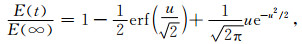
|
(5) |
The impulse response of the inline electric field can be obtained by differentiating equation (3)
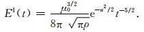
|
(6) |
The normalized step on and impulse transient responses of the homogeneous half-space are displayed in Figures la and lb, respectively, for values of resistivity of 0.3, 1, 10, 100 Ωm and 1000 Ωm. Both the transmitter (Tx) and the receiver (Rx) are on the surface and the offset is 1000 m. The solid lines indicate the analytic solutions in equations (5) and (6) stars indicate the results obtained by our 1D code. The agreement is very good.

|
Fig. 1 The normalized step on response (a) and the impulse response (b) of the homogeneous half-space for a range of resistivities of the half-space The solid lines indicate the analytic solution and the stars are the results obtained from our 1D code. |
We consider an 1D canonical model shown in Fig. 2, which consists of 0.3 Ωm sea water with varying depth hs, a 1 Ωm seafloor sediment, and a 100 m thick, 100 Ωm reservoir layer at a depth of hr below the seafloor. The inline electric field and its time derivative (impulse response) excited by a step on source signal were calculated by the recently developed 1D time domain code. Note that a unit source dipole is always used in the following analysis, unless stated otherwise.

|
Fig. 2 The 1D canonical reservoir model |
Fig. 3 shows the time derivative of the electric field response for five water depths (hs=100, 200 m, 300, 500 m and 1000 m) and the reservoir layer is at a depth of hr=1000 m below the seafloor. The horizontal electric dipole (Tx) is located at a height of 50 m above the seafloor and the receiver is at the seafloor. The transmitter (Tx)-receiver (Rx) offset is 4 km. The solid lines are the impulse response of the reservoir model with the resistive layer and the symbols are those of the background model (without the resistive layer). In the shallowest water (100 m depth), the impulse response of the reservoir model (red line) shows two peaks. The first one marks the arrival of the airwave and the second one the arrival of the field diffusing through the reservoir layer. This can be clearly seen when we compare it with the response of the corresponding background model (red stars). As sea water depth increases, the airwave arrives later and the amplitude becomes smaller-because of its decay in the deepening water layer. The presence of the airwave increases the electric field amplitude measured at receivers. When the water depth is 500 m, the impulse response of the reservoir model shows only one clear maximum. This means that the airwave and the signal from the deep resistivity layer arrive at about the same time, but one can still see a clear anomaly-compared to the background model. In deep water (1 km depth) the impulse response shows two peaks again, but the first one marks the arrival of the field diffusing through the reservoir layer and the second one the arrival of the airwave.

|
Fig. 3 Impulse responses for various water depths over the canonical 1D model as shown in Fig. 2 (solid lines) and the half-space without the reservoir (symbols) The transmitter is located at a height of 50 m above the seafloor and the transmitter-receiver offset is 4 km. The resistive layer is buried at hr=1000 m below the seabed. Even in the shallowest water (100 m, red) one can see a clear anomaly at around 1 s delay time. |
The time derivative of the electric field response is displayed in Fig. 4 for five offsets (1, 2, 3, 4 km and 6 km) in the shallow water (100 m depth) case. The source (Tx) is located at height of 50 m above the seafloor and the receivers are positioned at the seafloor. Again the reservoir layer is buried at a depth of hr=1000 m below the seafloor. At an offset of 1 km, the impulse response (blue line) of the reservoir model with the resistive layer is almost identical with that of the background model (blue stars) and the effect of the resistive layer is hardly recognizable. At an offset greater than 2 km, the effect of the deep resistive layer is clearly noticeable and one can see a clear anomaly compared to the background model. With the increase of the transmitter (Tx)-receiver (Rx) offset, the arrival of the target response shifts toward a later time and the amplitude of the response decreases. Fig. 5b shows the impulse response for a shallow target (hr=500 m). In comparison with the impulse response for the deep target (Fig. 4), one can observe that, as the depth of the reservoir layer gets shallower, the offset at which the effect of the resistive layer is recognizable gets smaller and the arrival of the target response comes earlier, and the amplitude of the target response gets bigger, so one can see a bigger anomaly.

|
Fig. 4 Impulse responses for various offsets over the canonical 1D model as shown in Fig. 2 (solid lines) and the half-space without the reservoir (symbols) The water depth is Hs=100 m and the transmitter is located at a height of 50 m above the seafloor. The resistive layer is buried at a depth of hr=1000 m below the seabed. From an offset of 2 km and greater, one can see a clear anomaly caused by the deep reservoir layer. |

|
Fig. 5 Step on response (a) and impulse response (b) for various offsets over the canonical 1D model as shown in Fig. 2 (solid lines) and the half-space without the reservoir (symbols) The water depth is hs=100 m and the transmitter is located at a depth of 50 m below the sea surface; The resistive layer is buried at a depth of hr=500 m below the seabed. |
In a marine CSEM survey, the horizontal electrical dipole source is often towed a few tens of meters above the sea floor and an array of receivers is positioned on the seabed. In this section, we investigate the possibility of using a surface-towed system in a shallow water survey. The horizontal electrical dipole source is towed at near the sea-surface and receivers may be towed at the sea surface behind the transmitter or positioned on the seafloor. One of the advantages of the surface-towed transmitter is that GPS recorders can be attached to the antenna to provide an accurate navigation. Tow speeds can be higher than for deep-towed transmitters, and no time is spent deploying and recovering instruments.
Here we present the transient response over the previously mentioned 1D canonical model (Fig. 2) for the deep reservoir target (hr=1000 m), but now the transmitter is moved to the sea surface and the receiver is located on the seabed or at the sea-surface. Fig. 6a shows the impulse response at an offset of 4 km in the shallow water case (100 m water depth). The blue line indicates the impulse response when both the transmitter and the receiver are located at the sea surface, and the red line indicates the impulse response when the transmitter is at the sea surface and the receiver is still on the seabed. The impulse response (green line) of the convenient deep-towed marine CSEM configuration (i.e., the transmitter is at a height of 50 m above the seabed and the receiver is on the seabed) is also illustrated. For comparison, the impulse responses of the backgrounding model without the resistive layer are also displayed (symbols). From Figure 6a, one can see that the early time impulse response curves of the three transmitter-receiver configurations are much different, while those at late times (t > 1 s) are almost identical in amplitude and shape and they fall together on the plot. One can see also that the anomalies of the three different configurations are very similar. The impulse response of the reservoir model (solid lines in Figure 6a) is divided by the corresponding response of the background model (symbols in Figure 6a) and illustrated in Figure 6b. One can see that the normalized responses of the three configurations are very similar in the shape and range. One gets the maximal anomaly, when both the transmitter and the receiver are located on the sea surface.

|
Fig. 6 The transient response of the 1D reservoir model (Figure 2) for the deep reservoir (hr=1000 m) in the shallow water (hs=100 m) The transmitter is moved to the sea-surface and the receiver is located on the seabed or the sea-surface. The sourceCTx)-receiver (Rx) offset is 4 km. (a) The impulse response; (b) The normalized field by the impulse response of the background model without the reservoir layer. |
In addition to the impulse response, Fig. 5a also shows the integrated, or step-on, response. This represents the measurement that would be made in practice, using a low frequency square wave transmission. Using this result, we can address several issues associated with practical applications, such as the switch-on speed required for the transmission current, the appropriate repetition rate for the transmission waveform, and the required signal to noise ratios for the receivers at various source-receiver offsets.
The noise threshold for seafloor electromagnetic receivers is around 10-15 to 10-14 V/(Am2) using a transmitter with a source dipole moment of around 100 kAm. Clearly, the expected signals are well above the noise, even for the larger source-receiver offsets. For all but the shortest source-receiver offset (1 km), the separation between the reservoir and no-reservoir case is discernible, from about a factor of 2 at 2 km offset to over half a decade at 6 km. In all cases the signal asymptotes to a late-time, DC response which is sensitive to the presence of the reservoir, but the transient response starting around 0.1 s has a larger separation between the reservoir and background, making the case for the time domain (versus DC resistivity) measurement.
The switch-on time for our EM transmitter was measured at about a millisecond over a 400A transition during a recent experiment using a 50 m antenna. Since the step on response does not rise above the noise floor until after 3~10 ms (depending on offset and, to a lesser extent, the noise floor chosen), and the separation between the background and target response does not develop until about 100 ms, this would appear adequate. Our transmitter uses bipolar transistors for switching, allowing a single transition between a negative peak current of -500 A and a positive peak current of 500 A to achieve a total transient of 1000 A. Some commercial transmitters using thy-ristor/SCR technology require an off state between polarities, but have larger peak current capabilities which compensates for the reduced step size. Except at the longest offset, the signal has reached the DC level by a few lO^s of seconds, suggesting that this would be an adequate repetition/stacking frequency.
For shallow water operations, as we have shown, seafloor receivers and transmitters do not provide significantly better resolution than surface systems. On the other hand, there are several logistical advantages of surface-towed systems. High transmission currents can be generated directly on the survey vessel, without the need to use high voltage transmission down a towing cable. Inline receiver antennas can be hundreds, rather than tens, of meters long to capture larger signals. Tow speeds can be increased from 1~2 knots to 4~6 knots (at a cost in stacking and/or spatial resolution). We have experimented with various towed electric field receiver systems, and have found that signal to noise ratios can be achieved which are no worse than a factor of 10 over deployed seafloor receivers. We are constructing a 150 kAm surface transmitter and have yet to measure the switching times we can achieve with this, although experience suggests they will not be significantly slower than those quoted above.
6 ConclusionsThis 1D study indicates that in both the shallow water and deep water environments, the airwave and the signal traveling trough the deep resistor arrive at different time. Although in an intermediate water depth the airwave and the signal from the deep resistivity layer arrive at about the same time, one can still see a clear anomaly compared to the background model without hydrocarbon reservoirs. For shallow water, deep-towing the transmitter near the seafloor has no clear advantage and a surface towed system may be used.
AcknowledgementsThis work was funded by BP America and the Scripps Seafloor Electromagnetic Methods Consortium. We would like to express our thanks to Katrin Schwalenberg and another anonymous referee for their constructive comments.
| [1] | Eidesmo T, Ellingsrud S, MacGregor L, et al. Sea Bed Logging (SBL), a new method for remote and direct identification of hydrocarbon filled layers in deepwater areas. First Break, 2002, 20: 144-152. |
| [2] | Weitemeyer K, Constable S, Key K, et al. First results from a marine controlled-source electromagnetic survey to detect gas hydrates off-shore Oregon. Geophysical Research Letters, 2006, 33: 629-632. |
| [3] | Cheesman S J, Edwards R N, Chave A D. On the theory of seafoor conductivity mapping using transient electromagnetic systems. Geophysics, 1987, 52: 204-217. DOI:10.1190/1.1442296 |
| [4] | Edwards R N, Chave A D. A transient electric dipole-dipole method for mapping the conductivity of the sea oor. Geophysics, 1986, 51: 984-987. DOI:10.1190/1.1442156 |
| [5] | Edwards R N.On the resource evaluation of marine gas hydrate deposits using seaoor transient electric dipole-dipole methods.1997, 62:63-74 |
| [6] | Yuan J, Edwards R N. The assessment of marine gas hydrates through electrical remote sounding:Hydrate without a BSR. Geophysicical Research Letters, 2000, 27: 2397-2400. DOI:10.1029/2000GL011585 |
| [7] | Schwalenberg K, Willoughby E, Mir R, et al. Marine gas hydrate deposits electromagnetic signatures in cascadia and their correlation with seismic blank zones. First break, 2005, 23: 57-63. |
| [8] | Ziolkowski A, Hobbs B A, Wright D. Multitransient electromagnetic demonstration survey in france. Geophysics, 2007, 72: 197-209. DOI:10.1190/1.2735802 |
| [9] | Stoyer C H. Electromagnetic fields of dipoles in stratified media. IEEE Transations on Antennas and Propagation, 1977, 25: 547-552. DOI:10.1109/TAP.1977.1141618 |
| [10] | Tang G M. Electromagnetic fields due to dipole antennas embedded in stratified anisotropic media. IEEE Transations on Antennas and Propagation, 1979, 27: 665-670. DOI:10.1109/TAP.1979.1142160 |
| [11] | Chave A, Cox C. Controlled electromagnetic sources for measuring electrical-conductivity beneath the oceans.1.forward problem and model study. Journal of Geophysical Research, 1982, 87(NB7): 5327-5338. DOI:10.1029/JB087iB07p05327 |
| [12] | Edwards R N. Marine controlled source electromagnetics:principles, methodologies, future commercial applications. Surveys in Geophysics, 2005, 26: 675-700. DOI:10.1007/s10712-005-1830-3 |
| [13] | Wannamaker P E, Hohmann G W, Filipo W A S. Electro-magnetic modeling of 3-dimensional bodies in layered earths using integral-equations. Geophysics, 1984, 49: 60-74. DOI:10.1190/1.1441562 |
| [14] | Chave A D. Numerical-integration of related hankel-transforms by quadrature and continued-fraction expansion. Geophysics, 1983, 48: 1671-1686. DOI:10.1190/1.1441448 |
| [15] | Newman G A, Homann G W, Anderson W L. Transient electromagnetic response of a three-diemnsional body in a layered earth. Geophysics, 1986, 51: 1608-1627. DOI:10.1190/1.1442212 |
| [16] | Anderson W L. Fast hankel-transforms using related and lagged convolutions. ACM Transactions on Mathematical Software, 1982, 8: 344-368. DOI:10.1145/356012.356014 |