 2010, Vol. 53


2. Institute of Geophysics, ETH Zurich, Zurich 8092, Switzerland
2. Institute of Geophysics, ETH Zurich, Zurich 8092, Switzerland
For DC resistivity problem involving 2-D inhomogeneities with 3-D sources, the initial simulation based on 3-D model could be transformed into the simulation based on a 2-D specified cross section of interest by the Fourier transform with respect to the strike, which is usually referred to 2.5-D simulation.After this transformation, an additional parameter is intro-duced which is called wavenumber.Transformed potentials for several wavenumbers should be calculated to obtain the total electric potentials in the space domain by the inverse Fourier transform.Several approaches have been successfully applied in 2.5-D DC resistivity numerical modeling problem.The integralequation technique[1] is efficient and accurate when a few regular inhomogeneities are buried in the model.The finite-difference method [2~4] is preferable because of its cheap implementation.The finite-element method[5] s a much popular tool since t can be easily combined with flexible model discretization strategies such as unstructured mesh.With the finite-element method, Fox et al.[6] and Tsourlos e tal.[7] made a systematical discussion about the effect of 2-D topography, respectively.An optimal algorithm to select the wavenumbers was presented by Xu et al.[8] to reduce the required number without losing accuracy.Based on this strategy, Pidlisecky and Knight[9] reported an efficient boundary condition and source singularity correction technique by which the modeling size could be greatly decreased.
Currently, for 2.5-D DC resistivity modeling with the finite-element method, models are often subdivided according to user's experiences.Moreover, the employed element types are regular[10, 11].Due to this, it becomes difficult to simulate complicated models.To avoid these problems, much attention has been paid to the adaptive finite-element technique[12, 13].Franke et al.[14] reported its application with unstructured mesh in 2-D magnetotelluric fields for arbitrary surface and seafloor topography.Li and Key[15] presented an adaptive finite-element algorithm used for 2-D marine controlled-source electromagnetic (MCSEM) modeling problem.For DC resistivity modeling problem, Ren and Tang[16] have given a distinctive adaptive finite-element algorithm involving unstructured mesh.
In this paper, we presented an adaptive finite-element technique for 2.5-D DC resistivity modeling.In this technique, a posteriol error estimator based on gradient recovery method is employed to make the node distribution more reasonable.Moreover, we utilize the irregular triangle to implement the subdivisions of arbitrary complex models.After that, a vertical contact model is simulated to compare the efficiencies of different adaptive strategies.Finally, two models: a 2-D inhomogeneity buried in the homogenous half space and a 2-D valley model are tested to validate our technique.
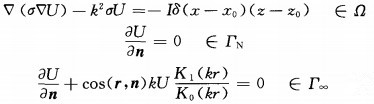
2 2.5-D DC Resistivity Modeling by the Finite-element MethodWe assume that the strike of the 2-D inhomogeneities is parallel to the y-axis in Cartesian coordinate system.The 2.5-D DC boundary value problem due to a single source point located on the earth surface in the wave number domain can be described as[17]
|
(1) |
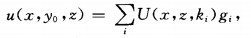
where σ denotes the electric conductivity in the modeling domain Ω, U is the transformed potential in the wave number domain, Iδ(x -x0)(z -z0。) is the source strength [17], r means a vector pointing to the outside boundary Γ∞ from the source point, r is its magnitude, ΓN denotes the earth-air interface on which Neumann-type boundary condition is enforced, K0 (kr) and K1 (kr) denote the zero-order and first-order modified Bessel function of the second kind, respectively, and k is called wavenumber.Once the transformed potential s observed, the total electric potential in the space domain can be obtained by the inverse Fourier
|
(2) |
where gi denotes the summation weight and u(x, y0, z) means the total electric potential on the profile y=y0.
After applying the Galerkin-weighed residual method[13] to every triangular element, all the element equations will be assembled into a global system as follows

|
(3) |
where K is a Nd×Nd matrix related to the known coordinates, U is the unknown vector of transformed nodal potentials, P is a Nd×1 vector only related to the function Iδ(x-x0)(z -z0) and Nd is the total number of nodes in the current mesh.
3 A-Posteriori Error EstimatorThe principal problem of the adaptive finite-element method is to find a suitable error est-mator.Different adaptive finite-element approaches are classified by d i fferent kinds of estimators.Generally, these error estimators can be divided into two categories: post-processing type[13] and residual based class[18, 19].The error estimator based on post processing introduced by Zienkiewicz and Zhu [20, 21] is used in our algorithm due to its simple implementation and robustness.
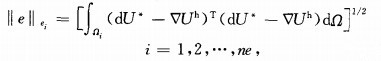
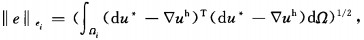
Since the analytical solutions are unknown for most of the cases, we approximately denote the numerical error in L2 norm for each elements, (For simplification, ||·||L2 is denoted by ||·||) by
|
(4) |
where Ωi means the area of the ith element, ▽Uh denotes the derivative of the finite-element solu-tion, super index h denotes h-type adaptive refinement which means only element size could be changedduringthe iterations, dU* is the recovered gradient[20] and ne is the total number of elements.Once dU* is obtained, every element error becomes available.
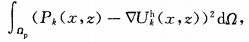
We adopt the Superconvergent Patch Recovery (SPR) technique proposed by Zienkiewicz and Zhu [20, 21] to obtain the recovered gradient.We fit the required recovered gradient described by a local continuous polynomial expansion of the function Pk(k -x, z), to the derivative of the finiteele-ment solution in a least-square sense.Usually, it s proper to set the order of the polynomial the same with that of the basis function[20].Thus, the least square fitting can be written into
|
(5) |
where

|
(6) |
Ωp denotes the element patch which consists of a set of elements selected surrounding a specified element in Ωp, ∇Ukh(x, z) denotesthe k-component of the derivative of the finite-element solution, ak, bk and ck are the unknown parameters used to determine the k-component of the recovered gradient.Through minimizing equation (5), we could obtain the system of equations

|
(7) |
where A is a 3×3 matrix related to the known coordinates in the element patch, 
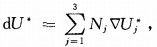
After solving the above equation, we can easily obtain each component of the recovered gradient ∇Uj* on arbitrary node j by substituting its coordinates into equation (6).Then the recovered gradient within each element could be expressed by
|
(8) |
where Nj(j=1, 2, 3) means the shape function defined in each llnear triangular element.Through substituting equation (8) into equation (4), element errorcouldbeeasily evaluated by using the numerical integral.
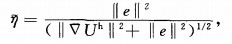
To predict the required new size for each element, we first define the relative L2 norm error for each element ei

|
(9) |
where ∇U denotes the analytical solution and ||∇Uh||ei is the derivative of the numerical potential in L2 norm.Then, we calculate the average element error η for all the elements introduced in the reference [16] to control the adaptive process.The adaptive refinement will terminate until η is less than the specified target value 
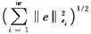
In an optimal mesh with the required target condition
|
(10) |

|
(11) |
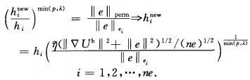
It is well known that standard finite-element method owns the following asymptotic convergence rate criteria at the element level[13]

|
(12) |
where p s the order of the basis function, λ s the strength of singularities andm in (p, λ) equals to λ when the element s in the singular regions, to p in the else regions.Wth this criterion and equation (11), we can easily give the relationship between the new element size predicted for the next mesh and the old element size in the current mesh
|
(13) |
Once each new element size is calculated, an automatic triangulation is performed until the terminal condition is satisfied.
4 Model DiscussionsIn this section, we make a systematical comparison about the efficiencies of different adaptive schemes.First, the efficiency of using transformed potential for each wavenumber as Uh mentioned in equation (4) to calculate the element error is addressed.Thus, the ith element error for each adaptive strategy can be written into

|
(14) |
where Umh denotes the transformed potential for the mth wavenumber in the wavenumber domain, dUm* means the evaluated recovered gradient and nw is the number of wavenumbers.After that, we select the best scheme for certain wavenumber to compare with another strategy
|
(15) |
here uh is the total electric potential in the space domain after the inverse Fourier transform defined in equation (2) and du* denotes the recovered gradient in this scheme.Finally, two additional models are tested to validate the efficiency and accuracy of our adaptive algorithm.
For each tested model, every surveying line is located on the profile y=0.Moreover, only a simple input file[22] consisting of initial model geometry information and attributes is needed.Some essential parameters are specified in our algorithm: element patch size Sp=5, the strength of the singularity λ=0.55 and a target relative error
We use a vertical contact model to make a systematical comparison about the efficiencies of different adaptive schemes.The vertical contact is located through the origin of the coordinate system.A resistivity ρ1=1 Ωm is assigned in the left half space and ρ2=100 Ωm in the right half space.The model has a size of 400 m×200 m (Fig. 1a).To discuss the accuracy, we adopt the pole-pole array with the single source point located at (-5.0 m, 0 m).The length of the surveying line is 10 m.The electrode spacing is 0.25 m.
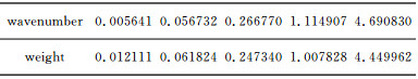
To choose the discrete wavenumbers suitable for this model, we adopt the algorithm proposed byXuetal.[8] for one source point existing case.Five wavenumbers and five corresponding weights are calculated for a set of specified measuring electrodes.
|
|
Table 1 Wavenumbers and weights used in Model 1 |
For the sake of amplification, we denote the strategy which uses the transformed potential for the ith wavenumber to calculate the element error by ki (i=1, 2, …, 5), respectively.Through comparing with the analytical solution[24], we plot the average relative error in apparent resistivity for the total measuring points as a function of the number of generated nodes in each rterative mesh in Fig. 1b.From this figure, it is seen that numerical results in the final meshes from the five different schemes can converge to the exact solution.However, strategy k5 with respect to the larger wavenumber seems to generate excessive nodes for such a small modeling domain, with little accuracy being improved compared with other strategies.Moreover, it does not converge as fast as the other four ones although more additional nodes have been inserted.The final meshes after one rteration for the five schemes are displayed in turn in Fig. 2.It s found that the elements near the source point have been greatly refined to eliminate the singularity.From the above discussion, it appears to show that the strategies with larger wavenumber can not handle the node distribution as well as the smaller ones.

|
Fig. 1 (a) Cross section of the vertical contact model; (b) Average relative errors in apparent resistivity as a function of the number of generated nodes from diferent strategies |

|
Fig. 2 (a) Initial mesh (282 nodes) which s the same for all the five strategies; (b) Final mesh (3220 nodes) for the scheme k1; (c) Final mesh (4140 nodes) for the scheme k2; (d) Final mesh (4588 nodes) for scheme k3; (e) Final mesh (4688 nodes) for scheme k4; (f) Final mesh (23167 nodes) for scheme k5 |
Based on the above discussion, we denote the adaptive procedure k1 corresponding to the smallest wavenumber by AP1.The adaptive scheme in which the element error s defined in equation (15) is called AP2.Both of the two schemes are described in Fig. 3.

|
Fig. 3 Flow chart of adaptive strategy AP1 and AP2 |
The relative errors in apparent resistivity calculated from the two adaptive schemes are displayed in Fig. 4.The strategy AP1 terminates after one iteration (Fig. 4a).It s obvious to see from these error curves that the accuracy is dramatically improved as the automatic refinement (Fig. 4b) is performed.The maximal relative error 17.15 % is observed near the source point in the initial mesh (282 nodes).As measuring electrode s moved far away from the source point, the error tends to be stable in the range of between 2 % and 4%.After one iteration (3220 nodes), the maximal relative error which appears in the vicinity of the source point has already been reduced to 0.93%.Moreover, the relative errors for other measuring points are considerably decreased with values no more than 0.69%.

|
Fig. 4 (a) Relative errors in apparent resistivity calculal^ed from adaptive scheme AP1; b) Element relative error in final generated mesh (3220 nodes) from AP1;(c) Relative errors in apparent resistivity calculated from AP2; (d) Element relative error in final generated mesh (4073 nodes) from AP2 |
For strategy AP2, the adaptive process also stops after one deration (Fig. 4c).In this scheme, the maximal relative error at the point near the source is decreased to 109% in the final mesh (4073 nodes).But the relative error indicates a visible increase along with the surveying line, which however, is not so obvious in AP1.Additionally, the average relative error for total measuring points in the final mesh is 0.42% in AP2, while it is 0.21 % in AP1.Moreover, the distribution of relative error within each element in the final meshes (Fig. 4b and Fig. 4d) also indicates that strategy AP1 is superior.Based on these results, we can conclude that both of the two schemes can be successfully performed in 2.5-D DC resistivity modeling.Considering both of the efficiency and accuracy, we adopt the procedure AP1 as our adaptive scheme.
4.2 Model 2The second model is a 2-D conducting inhomogeneous body (ρ1) buried in the half space (ρ0), which is shown in Fig. 5a.The computational domain has a size of 400 m×200 m.The cross section of the inhomogeneity has a size of 4 m×2 m.The buried depth is 2m.A very large resistivity contrast ρ1/ρ0=0.005 is designed.The dipole-dipole array with 13 electrodes s adopted.The dipole units specified as 1m.Unlike only one source point exists, we should recalculate a set of wavenumbers and weights for the two-source-point case to improve the accuracy.Here, we employ the program introduced by Pidlisecky and Knight[9] to select the optimal wavenumbers.The calculated results are listed in Table 2.Since the dipole source electrodes need to be moved, the whole adaptive algorithm should be repeated for all pairs of the source electrodes.

|
Fig. 5 (a) Cross section of a 2-D inhomogeneity buried in the homogenous half space; (b) Initial mesh (124 nodes); (c) Final mesh after one iteration (2055 nodes) |
|
|
Table 2 Wavenumbers and weights used in Model 2 |

To show the refinement process, we plot the rterative meshes when the source points are located at (-5 m, 0 m) and (-4 m, 0 m), respectively.For this case, the adaptive algorithm also terminates after one iteration.The initial mesh (124 nodes) and the final mesh after one iteration (2055 nodes) are depicted in Fig. 5b and Fig. 5c.These figures show that, the elements in the region near the source points have been automatically refined by which the superiority of using adaptive refinement has been revealed.To validate the observed dipole-dipole apparent resistivities, we compare them with the integral-equation modeling results proposed by Snyder[25].The relative errors in apparent resistivity for the initial mesh are shown in Fig. 6a and for final mesh after one iteration in Fig. 6b.Through comparison, a large average relative error 22.21% for the total measuring points is observed in the initial mesh.Surprisingly, through the refinement, the average relative error n the final mesh s reduced to 1.29%, by which the distinctive accuracy of our adaptive finite-element approach s demonstrated.

|
Fig. 6 Relative errors in apparent resistivity (a) in initial mesh, (b) in final mesh |
A 2-D valley model with 10 degree slopes is simulated (Fig. 3a).The resistivity of the valley is ρ0=100 Ωm.We employ the dipole-dipole array to analyze the topography effect.17 electrodes are arranged with 1 m spacing.The wavenumbers and weights in Model 2 are employed.Here, we give the mesh results when the dipole sources are located at (-8 m, 0 m) and (-7 m, 0 m), respectively.As we expect, this adaptive process only repeats once before achieving the terminal condition.We plot initial mesh (119 nodes) and final mesh after one iteration (2660 nodes) in Fig. 7b and Fig. 7c, respectively.Through these two figures, tt is seen that the refinement near the source points is highly performed.

|
Fig. 7 (a) Cross section of 2-D valley model; (b) Initial mesh (119 nodes); (c) Final mesh (2660 nodes) |
To verify our results, we compare the dipole-dipole apparent resistivities with integral-equation results presented by Oppliger[26].The relative errors in apparent resistivity for initial mesh are displayed in Fig. 8a and final mesh in Fig. 8b.After comparison, it is shown that the average relative error for the total measuring points in the initial mesh has a value of 19.09%.After one iteration, it has been remarkably decreased to 1 74%.However, we can observe through Fig. 8a and Fig. 8b that the distribution of the relative errors shows a slight asymmetry.This phenomenon may be explained by considering the selection of unstructured mesh.

|
Fig. 8 Relative errors in apparent resistivity obtained from (a) initial mesh and (b) final mesh |
We present a new algorithm to solve 2.5-D DC resistivity problem.Not only using the traditional finite-element method, an adaptive framework is applied to avoid adding any use's experiences about how to make model discretization reasonable into the simulation.A gradient-recovery-based a-posteriori estimator proposed by Zienkiewicz and Zhu[20, 21] (Z-Z) is adopted to predict a much more reasonable node distribution.The unstructured triangulation is used to flexibly subdivide the models.The tested models have given a good verification for our algorithm.It is seen from the visualized meshes, the singular regions such as near the source points are highly refined, while only a few nodes are inserted in other areas.This s a key to improve the accuracy and efficiency.
For the application of Z-Z error estimator to 2.5-D DC simulation which is typical scalar Helmholtz type, we give several satisfactory results by experiments.Its efficiency and strong robustness have been validated.
Although, only simple models are tested in this paper, its great potential to deal with much more complicated models with topography is expected.
AcknowledgmentsThe work is financially supported by the National High Technology Research and Development Program of China (2006AA06Z105, 2007AA06Z134).The authors show their great thanks to the three research teams who respectively present the high-quality solver LASPack, the powerful mesh visualization program MEDIT and the 2-D mesh generation package Triangle.Meanwhile, the authors really appreciate the precise work and warm suggestions from Prof.Zhao Guoze, Prof.Nikolay Palshin and Prof.Huang Qinghua when preparing this paper.Finally, we wish to thank two anonymous reviewers for their critical and professional comments.
| [1] | Hvozdara M, Kaikkonen P. The boundary integral solution of a DC geoelectric problem for a 2-D body embedded in a two-layered Earth. Journal of Applied Geophysics, 1996, 34: 169-186. DOI:10.1016/0926-9851(95)00013-5 |
| [2] | Mufti I R. Finite-difference resistivity modeling for arbitrary shaped two-dimensional structures. Geophysics, 1976, 41(1): 62-78. DOI:10.1190/1.1440608 |
| [3] | Dey A, Morrison H F. Resistivity modeling for arbitrarily shaped two-dimensional structures. Geophysical Prospecting, 1979, 27: 106-136. DOI:10.1111/gpr.1979.27.issue-1 |
| [4] | Mundry E. Geoelectrical model calculations for two-dimensional resistivity distributions. Geophysical Prospecting, 1984, 32(1): 124-131. DOI:10.1111/gpr.1984.32.issue-1 |
| [5] | Coggon H. Electromagnetic and electric modeling by finite-element method. Geophysics, 1971, 36(6): 132-155. |
| [6] | Fox R C, Hohmann G W, Killpacks T J. Topographic effects in resistivity and induced-polarization surveys. Geophysics, 1980, 45(1): 75-93. DOI:10.1190/1.1441041 |
| [7] | Tsourlos P I, Szymanskiz J E, Tsokas G N. The effect of terrain topography on commonly used resistivity arrays. Geophysics, 1999, 64(5): 1357-1363. DOI:10.1190/1.1444640 |
| [8] | Xu S Z, Duan B C, Zhang D H. Selection of the wavenumbersk using an optimization method for the inverse Fourier transform in 2.5D electrical modeling. Geophysical Prospecting, 2000, 48: 789-796. DOI:10.1046/j.1365-2478.2000.00210.x |
| [9] | Pidlisecky A, Knight R. FW2_5D:A MATLAB 2.5-D electrical resistivity modeling code. Computers & Geosciences, 2008, 34: 1645-1654. |
| [10] | Erdogan E, Demirci I, Candansay M E. Incorporating topography into 2D resistivity modeling using finite-element and finite-difference approaches. Geophysics, 2008, 73(3): 135-142. DOI:10.1190/1.2905835 |
| [11] | Ruan B Y. 2-D electrical modeling due to a current point by FEM with variation of conductivity within each triangular element. Guangxi Sciences, 2001, 8(1): 1-3. |
| [12] | Wiberg N E, Li X D, Abdulwahab F. Adaptive finite element Procedures in Elasticity and Plasticity. Engineering with Computers, 1996, 12: 120-141. DOI:10.1007/BF01299397 |
| [13] | Zienkiewicz O C, Taylor R L.The Finite-element Method (fifth edition) Volume I:The basic.Woburn, MA:Butterworth-Heinemann, 2000 Zienkiewicz O C, Taylor R L.The Finite-element Method (fifth edition) Volume I:The basic.Woburn, MA:Butterworth-Heinemann, 2000 |
| [14] | Franke A, B (O) rner R-U, Spitzer K. Adaptive unstructured grid finite element simulation of two-dimensional magnetotelluric fields for arbitrary surface and seafloor topography. Geophys.J.Int., 2007, 171: 71-86. DOI:10.1111/gji.2007.171.issue-1 |
| [15] | Li Y G, Key K. 2D marine controlled-source electromagnetic modeling:Part 1-An adaptive finite-element algorithm. Geophysics, 2007, 72(2): WA51-WA62. DOI:10.1190/1.2432262 |
| [16] | Ren Z Y, Tang J T.3D direct current resistivity modeling with an unstructured mesh by an adaptive finite-element method.Geophysics, 2009 (In press or web published) Ren Z Y, Tang J T.3D direct current resistivity modeling with an unstructured mesh by an adaptive finite-element method.Geophysics, 2009 (In press or web published) |
| [17] | Xu S Z. The Finite Element Method in Geophysics. Beijing: Science Press, 1994. |
| [18] | Ainsworth M, Oden J T. A unified approach to a-posteriori error estimation using element residual methods. Numer.Math., 1993, 65: 23-50. DOI:10.1007/BF01385738 |
| [19] | Ainsworth M, Oden J T.A Posteriori Error Estimation in the Finite Element Analysis.New York:John Wiley, 2000 Ainsworth M, Oden J T.A Posteriori Error Estimation in the Finite Element Analysis.New York:John Wiley, 2000 |
| [20] | Zienkiewicz O C, Zhu J Z. Super-convergent patch recovery and a posteriori error estimates.Part 1:the recovery techniqu. Int.J.Numer.Methods Eng., 1992, 33(2): 1331-1364. |
| [21] | Zienkiewicz O C, Zhu J Z. Super-convergent patch recovery and a posteriori error estimates.Part 2:error estimates and adaptivity. Int.J.Numer.Methods Eng., 1992b, 33(3): 1365-1382. |
| [22] | http://www.cs.cmu.edu/-quake/triangle.html, assessed March 12, 2007. http://www.cs.cmu.edu/-quake/triangle.html, assessed March 12, 2007. |
| [23] | Frey P J.MEDIT-an interactive mesh visualization software.http://www-rocq.inria.fr/gamma/medit/medit.html, accessed November 26, 2007. Frey P J.MEDIT-an interactive mesh visualization software.http://www-rocq.inria.fr/gamma/medit/medit.html, accessed November 26, 2007. |
| [24] | Fu L K. Lecture of Geoelectrical Prospecting Methods. Beijing: Geological Publishing House, 1983. |
| [25] | Snyder D D. A method for modeling resistivity and IP response of two-dimensional models. Geophysics, 1976, 41(4): 997-1015. |
| [26] | Oppliger G L. Three-dimensional terrain corrections for mise-à-la-masse and magnetometric resistivity surveys. Geophysics, 1984, 49: 1718-1729. DOI:10.1190/1.1441579 |