 2010, Vol. 53


In transient electromagnetic (TEM) surveys with a rectangular large loop, to avoid the effects of lateral inhomogeneities[1] and simplify discussion[2], It is usually required to collect induced voltage in the central part the loop. As a result, one may invert the TEM data by the theory of circular loop[3]. However, in tield, to enhance work efficiency, the induced voltage will be measured rather close to the wire. In this case, the interpretation theory of central loop will fail[4]. Thus, there is a great demand of an inversion to interpret the near loop measurements.
Occam's inversion initiated by Constable et al[5] has been adapted by Weng et al. [6] to meet the requirement. And during the inversion, an important thing is to develop a rapid and accurate modeling scheme for a rectangular loop.
In fact, the TEM response from a large rectangular loop, over a layered ground, had been evaluated by Poddar[7], Raiche[4] and Goldman and Fitterman[8]. In their ways, firstly, the response in frequency domain was computed by integrating the fields from current dipoles along the loop, or vertical magnetic dipoles that spans the loop surface, and then time-domain response was obtained through G-S transform from he frequency results[9, 10]. In the former case, an improper integral (Hankel transform) and a finite integral over the loop are required; in the latter method, due to the asymmetry of the source, one has to perform a two-dimensional Fourier transform[11, 12].
To speedup the computation, Sorensen and Christensen expressed the fields from the finite electrical dipole by Hankel transforms and as integral of Hankel transforms, and extended the theory of fast Hankel transform to include integral of Hankel transforms[13]. The key of the method is to calculate the filter coefficients, which, however, will depend on transmitter-receiver separation.
In the paper, we introduce a new method, in which a rectangular loop is spanned by a certain number of squares of finite dimensions rather than infinitely small dipoles. Accordingly, the responses from a rectangular loop are the summation of the fields from all these fictitious squares, which could be approximated by circular loops of the same transmitting area as that of the squares to calculate the electromagnetic fields. To enhance the computation efficiency, the responses from each circular loop are firstly summed up in frequency domain. By doing so, the frequency responses from a rectangular loop can still be approximated by standard Hankel transforms, while the summation is acted upon the Bessel functions involving the distances from the receiver to each square center and incorporated into the kernel function of the transform. The time domain response can then be computed from the responses in frequency domain through cosine transform[14, 15]. The accuracy of the method depends on the approximation of square with circular loop. Numerical results in the paper show a relative error of less than 10-3 of the approximation comparing with analytical results.
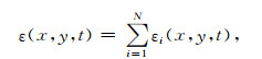
2 PrincipleThe fields from a rectangular loop source over ground can be exactly calculated by adding all the fields from the fictitious squares that overlay each other by sides to span the rectangular loop (Fig. 1). With this assumption, the induced voltage ε(x, x, t) at point (x, y) after a delay time t from the current shutoff can be expressed as where εi(x, x, t) is the voltage generated by the square centered at position (xi, yi). N is the total number of the squares spanning the rectangular loop. Ostensibly, the summation in equation (1) can be done directly in time domain. However, we do t in an alternate way as following.
|
(1) |

|
Fig. 1 Square summation principle in which a rectangular loop is spanned by a certain number of fictitious squares |
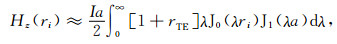
Firstly, we approximate in frequency domain, the vertical magnetic field from a square loop at the ground surface by that from a circular loop, and after Patra and Mallick[14], the vertical magnetic field is written as
|
(2) |
where I is current strength, a is the equivalent loop radius which can be estimated from side length i of a square by 
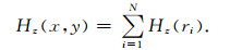
As a rectangular loop will be spanned by N squares, the magnetic field Hz(x, y) from the loop can be written as
|
(3) |
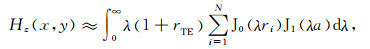
Substituting equation (2) into equation (3), and exchanging integration and summation, we have
|
(4) |
In equation (4), the right hand is in fact a standard Hankel Transform, that is

|
(5) |
where
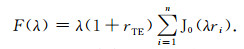
|
(6) |
From equation (5), it can be seen that the approximate field can be evaluated by Hankel transform only once; while the summation over the fields from all squares is incorporated into the integrand with the form of Bessel function addition; thus significantly speedups the computation of the response from a rectangular loop. In our program, we adapted the coefficients of Hankel transform filter from Piao to evaluate equation (5)[18].
Once the frequency responses are obtained, the time responses of a rectangular loop can be calculated through cosine transform[14, 15], while the induced voltage can be calculated by forward difference from the time responses.
3 Results and DisccussionsThe TEM response from a rectangular loop over a homogeneous half space is of closed form[19] and will be used to verify the accuracy of the new method as in Fig. 2, where the resistivity of the ground is 100 Ωm. The responses at the center of the loops with side length varying from 200 m to 1000 m are calculated. The squares used to span all the loops are 50 m by 50 m, so that, a loop of 200 m × 200 m will be replaced by 16 squares. From Fig. 2, it can be seen that approximate responses coincide quite well with the analytical signals, indicating a high accuracy of the method. Meanwhile, given a square, the larger a loop size is, the more the squares will be needed. If the loop was large enough, for instance, of 1000 m border length, the squares could be so small that they could be considered as vertical magnetic dipoles. At this point, our method returns to the magnetic dipole equivalence method.

|
Fig. 2 Induced voltage by square summation method compared with theoretical response of a half space generated by loops of different side length |
A more typical example is shown in Fig. 3. The loop in Fig. 3a is of a width-length ratio of 3, thus it is very narrow and can not be mimic by a circular loop. Three different stations, O1 at (40, 40), O2 at (300, 40) and O3 at (300, 100), are specified on purpose to represent extreme positions. The three-layered model at the right panel of Fig. 3a will be energized by the loop to generate TEM responses shown in Fig. 3b. One can see that at late time, the different responses at the stations overlay each other. However, at early time, the responses vary with position; the closer the station is to the border, the weaker the early response is. In fact, at late time, due to the mutual induction, the eddy currents are homogenized over half space, so that there will be no difference in the fields at earth surface[12]. However, at early time, the field distribution will be shaped by the loop, resulting in a spatial dependence.

|
Fig. 3 (a) Different positions in rectangular loop (left) over a three-layered earth (right). (b) Shows the induced voltages at the stations in (a), while (c) plots the whole-time apparent resistivity from the responses in (b) |
From the responses, whole-time apparent resistivity can be calculated[20, 21]. Here, we adapt the method by Zhang et al. [22]. To avoid the non-uniqueness of the solution, during the whole-time apparent resistivity calculation, rock sample measurements or other prioti geophysical information will be utilized to set the initial guess to get the solution of the first few time windows; after that, use the solution as the initial solution to the later time channel consecutively until meeting the last time window. Fig. 3c illustrates the results, from which one can see that the whole-time resistivity curves of the three points overlay each other and reveal the true resistivity distribution. Because in calculating the whole-time apparent resistivity, the responses at different positions will try to fit to analytical results. Therefore, the coincidence implies that the responses from the new method are almost the same as the analytical signals. This again highlights the accuracy of our method.
A real TEM survey with rectangular loop in a coal mine is depicted Fig. 4. The loop was 760 m by 800 m. Current frequency was 32 Hz, and receiving moment was 104 m2. The data were recorded using GDP-32Ⅱ in the portion symbolized by cross. Induced voltages were sampled from 50 μs to 50 ms at all stations. An example of the voltage and the corresponding apparent resistivity are shown in Fig. 5. The resistivity near the earth surface is as low as 10 Ωm, and increases with depth to about 100 Ωm.

|
Fig. 4 A field TEM survey using a large rectangular loop |

|
Fig. 5 Induced voltage and apparent resistivity of the station at the most left-top corner of the loop |
The TEM responses are inversed by the adapted Occam’s inversion[6], and the results are shown in Fig. 6 and Fig. 7. In Fig. 6, the resistivity sections along Line 8 and Line l3 both reveal two resistivity low abnormals at the depth of about 150 m. According to the local geology, the abnormal relate to the sinks due to the collapses of overburden. To illustrate the 3D distribution of the sinks, the resistivity volume was sliced at different depths shown in Fig. 7. In deep region, there exist four sink centers, which could be connected through narrower tunnels. The overall shape reflects the mined area. Near the surface, the low abnor-mals disappear, which means that the collapse happened under the ground.

|
Fig. 6 Resistivity section along Line 8 and Line 13 in Fig. 4 |

|
Fig. 7 Resistivity slices at different depth inversed from the data in Fig. 4 |
The new method allows for a fast computation of transient responses from a rectangular loop over a layered earth. The error stems from the approximation of a square loop by a circular loop. The relative error is less than 10-3 when at least 16 squares are used to span a loop. During the computation, both Hankel transform and cosine transform are executed only once, thus the method has great computation efficiency, making the inversion of large loop TEM in Held possible. Meanwhile, as the response of a station very close to the loop could be estimated accurately, one can interpret the induced voltage measured near the loop, thus expanding greatly the survey range which used to be limited to the central part of the loop of about l/3 loop length, significantly enhancing the productivity of data collecting with large loop sources.
AcknowledgementsThe research is support-ed by the National Science Foundation of China (40874050). We also appreciate the valuable suggestions from anonymous reviewers and Prof Egbert in Oregon State University.
| [1] | Partra H P. Central frequency sounding in shallow engineering and hydro-geological problems. Geophysical Prospecting, 1970, 18(2): 236-254. DOI:10.1111/gpr.1970.18.issue-2 |
| [2] | Krivochieva S, Chouteau M. Whole-space modeling of a layered earth in time-domain electromagnetic measurements. Journal of Applied Geophysics, 2002, 50(2): 375-391. |
| [3] | Singh N P, Mogi T. Electromagnetic response of a large circular loop source on a layered earth:a new computation method. Pure appl.Geophys., 2005, 162(1): 181-200. DOI:10.1007/s00024-004-2586-2 |
| [4] | Raiche A P. Transient electromagnetic field computation for polygonal loops on layered earths. Geophysics, 1987, 52(6): 785-793. DOI:10.1190/1.1442345 |
| [5] | Constable S C, Parker R L, Constable C G. Occam's inversion:a practical algorithm for generating smooth modes from electromagnetic sounding data. Geophysics, 1987, 52(2): 289-300. |
| [6] | Weng A H, Gao L L, Liu Y H. Inversion of TEM data from rectangular loop on a layered earth model. Computing Techniques for Geophysical and Geochemical Exploration (in Chinese), 2008, 30(4): 314-316. |
| [7] | Poddar M. A rectangular loop source of current on a multilayered earth. Geophysics, 1983, 48(1): 107-109. DOI:10.1190/1.1441398 |
| [8] | Goldman M M, Fitterman D V. Direct time-domain calculation of the transient response for a rectangular loop over a two-layer medium. Geophysics, 1987, 52(7): 997-1006. DOI:10.1190/1.1442368 |
| [9] | Knight J H, Raiche A P. Transient electromagnetic calculation using the Gaver-Stehfest inverse Laplace transform method. Geophysics, 1982, 47(1): 47-50. DOI:10.1190/1.1441280 |
| [10] | Luo Y Z, Chang Y J. A rapid algorithm for G-S transform. Chinese J.Geophys, 2000, 46(43): 684-690. |
| [11] | Lee T, Lewis R. Transient response of a large loop on a layered ground. Geophysical Prospecting, 1974, 22(3): 430-444. DOI:10.1111/gpr.1974.22.issue-3 |
| [12] | Nabighian M N.Electromagnetic Methods in Applied Geophysics, Volume 1, Theory.Tulsa:Society of Exploration Geophysicists, 1988 Nabighian M N.Electromagnetic Methods in Applied Geophysics, Volume 1, Theory.Tulsa:Society of Exploration Geophysicists, 1988 |
| [13] | Sørensen K I, Christensen N B. The fields from a finite electrical dipole-a new computational approach. Geophysics, 1994, 59(6): 864-880. DOI:10.1190/1.1443646 |
| [14] | Patra H P, Mallick K.Geosounding principles 2:time varying geoelectric sounding.Amsterdam, Elsevier Scientific Publishing Company, 1980 Patra H P, Mallick K.Geosounding principles 2:time varying geoelectric sounding.Amsterdam, Elsevier Scientific Publishing Company, 1980 |
| [15] | Li J S, Piao H R. On the calculation and application of the apparent resistivity of transient EM sounding by electric dipole. Computing Techniques for Geophysical and Geochemical Exploration (in Chinese), 1993, 15(2): 108-116. |
| [16] | Das U.A reformalism for computing frequency-and time-domain EM responses of a buried, finite-loop.SEG Annual Meeting Abstracts, Houston, TX, 1995.811-814 Das U.A reformalism for computing frequency-and time-domain EM responses of a buried, finite-loop.SEG Annual Meeting Abstracts, Houston, TX, 1995.811-814 |
| [17] | Weng A H, Li Z B, Wang X Q. Magnetic field computation for large loop source. Computing Techniques for Geophysical and Geochemical Exploration (in Chinese), 2000, 22(3): 245-249. |
| [18] | Piao H R. The Theory of Electromagnetic Sounding Methods. Beijing: Geological Publishing House, 1990. |
| [19] | Nabighian M N, Oristaglio M L. On the approximation of finite loop sources by two-dimensional line sources. Geophysics, 1984, 49(7): 1027-1029. DOI:10.1190/1.1441717 |
| [20] | Bai D H, Maxwell a m, Lu J, et al. Numerical calculation of all-time apparent resistivity for the central loop transient electromagnetic method. Chinese J.Geophys, 2003, 46(5): 697-704. |
| [21] | Wang H J. Time domain transient electromagnetism all time apparent resistivity translation algorithm. Chinese J.Geophys, 2008, 51(6): 1936-1942. |
| [22] | Zhang C F, Weng A H, Sun S D, et al. Computation of whole-time apparent reisistivity of large rectangular loop. Journal of Jilin University (Earth Science Edition), 2009, 39(4): 755-758. |