 2010, Vol. 53


At present, 3D MT forward modeling and inversion is the highlight. However, because of the complexity and lack of computing power in 3D inversion, 1D and 2D inversion methods are commonly used to solve the most practical problem, and 2D inversion methods are more popular. For 2D inversion, how to get the rapid and stable inversion results and the clearer geoelectrical interfaces are still the research focus. Predecessors introduced lots of methods in how to improve the speed and the stability of the inversion, such as;OCCAM inversion provided by Constable[1] and deGroot-Hedlin[2];RRI provided by Smith and Booker[3]; REBOCC provided by Siripunvaraporn and Egbert[4];NLCG provided by Rodi[5], ABIC method provided by Ogawa[6] and Uchida[7], and so on. At the same time, experts have proposed and developed the Monte Carlo method, artificial neural net[8], simulated annealing (SA)[9] and multiresolution inversion[10] in China. These methods often introduce model objective function based on the smoothest stable functional,so the results are much smooth and couldn’t represent the geo-electrical interface clearly which make it difficulty in the geophysical and geological interpretation. Thus sharp boundary inversion is being researched by more and more experts.
The most famous method in sharp boundary inversion is provided by de Groot-Hedlin[11]. This method represents the earth subsurface in terms of 2D model consisting of a limited number of layers with laterally varying thickness in each survey point and each layer having uniform resistivity. The inversed parameters are the resistivity and the depths of each layer under each survey point. In order to make the inversion stable and avoid the false structures, the differences in the resistivity between adjacent layers and the lateral variation in layer depth are both penalty. This inversion method is effective for layer models. However, the method requires number of layers before the inversion starting, so if the priori information isn't correct, the result will be incorrect. It also has the Hmitation in block body inversion and is hiconvenient to calculate the sensitivity matrix. Meanwhile, Farquharson used L1 norm to solve this problem[12]. It represents the clear electrical interface in the result, but the boundary can7 t be accurately positioned and the shape of block bodies often has a distortion. Therefore it is hard to be used in the practical application.
The focusing inversion method[13~15] based on the minmum gradient support functional offers a path to solve the problem how to display the electrical interface clearer. Liu[16, 17] developed it and makes it reflect a relative superiority on solving the sharp boundary inversion. However, in general focusing inversion only vertical and horizontal direction gradient will be calculated, the characterization of the oblique electrical interface will lack of representation. In the basis of focusing inversion, we analyze the construction of the objective function by taking 45° and 135° diagonal gradient support into consideration and study a new inversion method to represent the clearer and more accurate oblique geo-electrical interface.
2 Algorithm 2.1 Model constructionUsing vertical division lines along surveyed line direction depending on the interval distance of the surveyed points or at your will, the horizontal division lines along depth direction which may be set enough dense and fixed to satisfy the modeling into many rectangle units in accordance with its property distribution. If the values of resistivity of each unit are filled, then its MT field response produced on the earth's surface can be calculated. The inversed parameters are resistivity in each unit: model=(ρ1,ρ2,ρ3,…,ρn-1,ρn). Where ρ is resistivity, n is the number of the units.
2.2 Forward modeling and sensitivity matrix calculationNumerical computing of MT forward modeling procedure is realized using finite elements method[18, 19], which coincides with the division of model construction.
To speed up the calculation of the sensitivity matrix for 2-D MT inversion using finite elements, the principle of electromagnetic reciprocity is applied[20, 21]. The governing relationship for the Jacobians of the field along strike is obtained by differentiating the Helmholtz equation with respect to the conductivity of each region in the finite element mesh. According to the principle of electromagnetic reciprocity, the roles of sources and receivers are interchangeable. Utilizing reciprocity theorem, the field values obtained from the original forward problem and for new unit sources imposed at the receivers are then utilized in the calculation of the Jacobian matrix by simple multiplication and summation with finite-element terms at each rectangle in the mesh. Reciprocity decreases the computational expense of Jacobian matrix to the order of the number of stations of interest.
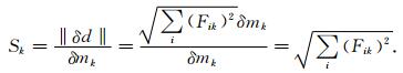
2.3 Definition of the weighting matrices for the model parameters and data[22]To solve the sensitivity of the data to the perturbation of one specific parameter mk,we apply the relationship between variational data δdi and variational modil parameter δmk;δdi=Fikδmk, and Fik are the elements of Frechet matrix.
So the integrated sensitivity Sk of the data to the parameter mk as the ratio can be determined:
|
(1) |
And the diagonal matrix with the diagonal elements equal to Sk is called an integrated sensitivity matrix S;S=

We identify a weighting matrix for the model parameters as the diagonal integrated sensitivity matrix;Wm=[Wj]=[Sj]=S. Thus we can introduce the weighted model parameters as: mw=Wmm.
Using these notations, the inverse problem can be written as: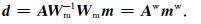
Thus a new integrated sensitivity will be calculated as:

|
(2) |
Therefore, data are uniformly sensitive to the new weighted model parameters.
In the similar way,we can define the diagonal data weighting matrix as: 
In order to reduce the computation,the weighting matrices are calculated only once and then they keep unchanged.
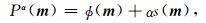
2.4 The theory of sharp boundary uiversion base on minimum gradient support 2.4.1 Theory of regularization problem[23, 24]In geophysical inversion, in order to solve the problem of stable and non-uniqueness, the regularization theory is introduced:
|
(3) |
where, m is model, φ(m) is data misfit functional, s(m) is model objective functional, Pα (m) is parametric objective function, α is the regularization factor.
2.4.2 Theory of focusing inversion method[13~15]The objective function of focusing inversion could be written as:

|
(4) |
where d is data,A(m) is the result of forward modeling.
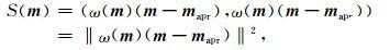
The stabilizing S(m) is:
|
(5) |
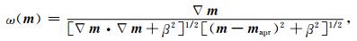
where
|
(6) |
is the matrix elements of the minimum gradient support functional, Vm is the gradient of model, β is a small number, m and mapr are model parameters andpriori model parameters,respectively.
The property of the minimum gradient support functional can be used to increase the resolution of blocky structures. For the effect of gradient support, the minimum gradient support functional could help to generate a sharp and focused image of the inverse model. Fig. 1 illustrates this property of the minimum gradient support functional.

|
Fig. 1 Effect of the gradient support |
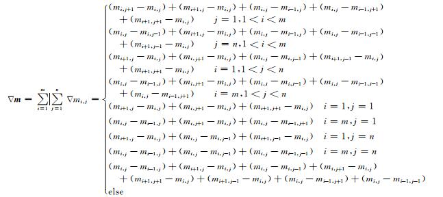
In a general focusing inversion, only vertical and horizontal direction gradient will be calculated. In this paper, we calculate the 45° and 135° diagonal gradient support (Fig. 2) and add it to the minimum gradient support functional. Thus the oblique geo-electrical interface could be represented clearer and better.

|
Fig. 2 Direction of diagonal gradient |
The mesh comprises m × n cells. Thus the gradient of model could be modified as:
|
And Fig. 2 shows the direction of the diagonal gradient.
2.5 Solving minimum of the objective functional by RCGRegularized conjugate gradient (RCG) method[22, 25~28] is used to solve the objective functional minimum. This procedure insures the convergence of the inversion and enhances the stability and speed of inversion calculation.
The main scheme of RCG method is as follows:
Suppose m is model parameters, n is the iteration number, and
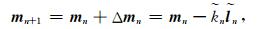
|
(7) |
where 

To determine 

|
(8) |
where d is data,A (m) is result of forward modeling, Fm s the Frechet matrix, We s a matrix of the stabilizer.
Thus, 
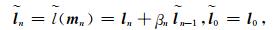
|
(9) |
where 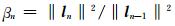
The expression of the step length 
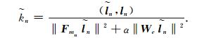
|
(10) |
Thus, the model will be updated until we get an acceptable result. We can also limit the range of the model parameters to avoid the case of divergence and make the iteration more stable.
3 Synthetic Model Test 3.1 Oblique boundary modelFig. 3a is the designed model representation. Some of the inversion parameters are: 12 frequencies points (0.01,0.03, 0.1, 0.3, 1, 3, 5, 10, 15, 30, 50, 100 Hz), the mesh comprises 58 X 40 cells. The initial model is the half space whose resistivity is 500 Ωm.

|
Fig. 3 Oblique boundary model and inversion results (a) Designed model;(b) Inversion result of SBI by adding diagonal gradient support;(c) Inversion result of smoothest inversion. |
After 10 iterations, the overall objective function of our result satisfies the accuracy with the value of 0.01015, and it is illustrated in Fig. 3b. Comparing with smoothest inversion (OCCAM inversion) in Fig. 3c, although the RMS of the OCCAM inversion is 0.01201, which is similar with our result, after same iterations, we can find that the geo-electrical interface is more clearly revealed.
3.2 Triangle modelThe model s shown in Fig. 4a. It is the same example as Ref. [12]. The mesh comprises 80×65 cells and extends from -12 km to 12 km in the horizontal direction and from -12 km to 10 km in the vertical direction (the earth-air interface at 0). The central mesh comprises 60 × 40 cells and extends from -5 km to 5 km in the horizontal direction and from 0 km to 5 km in the vertical direction. The shape of the blocky body is isosceles right triangle, the vertical right-angle edge extends from 0.5 km to 2.5 km and the horizontal one extends from -0.5 km to 1.5 km. Smoothest inversion (Fig. 4b) and sharp boundary inversion (Figs. 4c, 4d) all use the data which comprises apparent resistivity and impedance phase of the E-polarization at 12 frequencies points as the former example. Gaussian random noise of standard deviation equal in magnitude to 1% of a datum is added to make the data set that s to be inverted. The 100 Ωm half space is used as initial model and the range of the value of model parameters is from 0 to 500 Ωm.

|
Fig. 4 Triangle model and inversion results (a) Model according to Ref.[11]; (b) Inversion result of smoothest inversion; (c) Inversion result of SBI by adding diagonal gradient support;(d) Inversion result of SBI without diagonal gradient support;(e) Datamisfk error curve with iteration;(f) Overall objective function curve with iteration. |
Fig. 4b shows the boundary of the blocky body in the result of smoothest inversion (OCCAM inversion). It exists a false image. Farquharson (2008)[12] has used L1 norm to solve this model, the result shows that the electrical interface is clear, however, the shape of the blocky body is distorted so that it can't be shown as isosceles right triangle. Comparing with smoothest inversion,the result of the inversion based on the method in this paper (Fig. 4c) seems better. The geo-electrical interface is clearer and the blocky body can be distinguished. Meanwhile, comparing with the result in Farquharson's paper, the boundary of the result is as clear as Farquharson's result, moreover, the shape of the inversed blocky body of our result isn't distorted, each edge is accurate positioned. At the same time, we do the inversion by adding diagonal gradient support and without diagonal gradient support (Fig. 4d). The figures have shown the difference between them. The result adding diagonal gradient support has the better effect in representing the oblique geoelectrical interface.
Fig. 4e and Fig. 4f are data misfit error curve and overall objective function curve with iterative numbers for result of SBI by adding diagonal gradient support. After 20 iterations, values are about 0.01 and 0.05 respectively. It is smaller than the value of OCCAM inversion which are 0. 03 and 0. 075 after 20 iterations. Therefore, the result of SBI by adding diagonal gradient support can fit the needs of inversion.
The complex models are also used to test this algorithm, and the results show that the algorithm in this paper is effective in these models.
4 ConclusionBased on the theory of focusing inversion, we introduce the diagonal gradient support to the model objective functional. The algorithm can make the geo-electrical interface and the blocky body be shown clearer and more accurate, and t s also stable during inversion. Thus the problem that the oblique geo-electrical interface couldn't be inversed clear in the general MT inversion could be solved. Some models are designed to test the feasibility and efficiency of this algorithm. In accordance with the results, we can know the algorithm could really improve the representation of the oblique geo-electrical interface compared with the results of smoothest inversion and published papers. And it provides a path to solve this problem in practical application.
AcknowledgmentsThanks for the financial support of National High Technology Research and Development Project (863) (2008AA093001), National Science and Technology Major Project (2008ZX05005-005-010HZ), the National Natural Science Foundation of China (40674063), National Key Foundation Research Developing Projett (973) (2007CB411706-02) & (2007CB411702) and Projett (MG20080103) of State Key Laboratory of Marine Geology, Tongji University.
| [1] | Constable S C, Parker R L, Constable C G. Occam's inversion:a practical algorithm for generating smooth models from electromagnetic sounding data. Geophysics, 1987, 52(3): 289-300. DOI:10.1190/1.1442303 |
| [2] | deGroot-Hedlin C, Constable S. Occam's inversion to generate smooth, two-dimensional models from magnetotelluric data. Geophysics, 1990, 55(12): 1613-1624. DOI:10.1190/1.1442813 |
| [3] | Smith J T, Booker J R. Rapid inversion of two-and three-dimensional magnetotelluric data. J.Geophys.Res., 1991, 96: 3905-3922. DOI:10.1029/90JB02416 |
| [4] | Weerachai Siripunvaraporn, Gary Egbert. An efficient data-subspace inversion method for 2-D magnetotelluric data. Geophysics, 2000, 65(3): 791-803. DOI:10.1190/1.1444778 |
| [5] | Rodi W, Mackie R L. Nonlinear conjugate gradients algorithm for 2-D magnetotelluric inversion. Geophysics, 2001, 66(1): 174-187. DOI:10.1190/1.1444893 |
| [6] | Ogawa Y, Uchida T. A two-dimensional magnetotelluric inversion assuming Gaussian static shift. Geophys.J.Int., 1996, 126: 69-76. DOI:10.1111/gji.1996.126.issue-1 |
| [7] | Uchida T. Smooth 2-D inversion for magnetotelluric data based on statistical criterion ABIC. J.Geomag.Geoelectr., 1993, 45: 841-858. DOI:10.5636/jgg.45.841 |
| [8] | Wang J Y. Review of electrical prospecting for petroleum in China. Progress in Exploration Geophysics, 2006, 29(2): 77-82. |
| [9] | Yang H, Wang J L, Wu J S, et al. Constrained joint inversion of magnetotelluric and seismic data using simulated annealing algorithm. Chinese J.Geophys, 2002, 45(5): 723-734. DOI:10.1002/cjg2.v45.5 |
| [10] | Xu Y X, Wang J Y. A multiresolution inversion of one-dimensional magnetotelluric data. Chinese J.Geophys, 1998, 41(5): 704-711. |
| [11] | de Groot-Hedlin C, Constable C, et al. Inversion of magnetotelluric data for 2D structure with sharp resistivity contrasts. Geophysics, 2004, 69(1): 78-86. DOI:10.1190/1.1649377 |
| [12] | Farquharson C G. Constructing piecewise-constant models in multidimensional minimum-structure inversions. Geophysics, 2008, 73(1): 1-9. |
| [13] | Portniaguine O, Zhdanov M S. Focusing geophysical inversion images. Geophysics, 1999, 64: 874-887. DOI:10.1190/1.1444596 |
| [14] | Portniaguine O, Zhdanov M S. 3-D magnetic inversion with data compression and image focusing. Geophysics, 2002, 67(5): 1532-1541. DOI:10.1190/1.1512749 |
| [15] | Zhdanov M S, Ellis R, Mukherjee S. Three-D regularized focusing inversion of gravity gradient tensor data. Geophysics, 2004, 69: 925-937. DOI:10.1190/1.1778236 |
| [16] | Liu X J.Focusing inversion images of magnetotelluric data[Ph.D.thesis] (in Chinese).Shanghai:Tongji University, 2007 Liu X J.Focusing inversion images of magnetotelluric data[Ph.D.thesis] (in Chinese).Shanghai:Tongji University, 2007 |
| [17] | Liu X J, Wang J L, Chen B, et al. Discussion on focus inversion algorithm of 2-D MT data. Oil Geophysical Prospecting, 2007, 42(3): 338-342. |
| [18] | Coggon J H. Electromagnetic and electrical modeling by the finite element method. Geophysics, 1971, 36(1): 132-155. DOI:10.1190/1.1440151 |
| [19] | Wannamaker P E, Stodt J A, Rijo L. A stable finite-element solution for two-dimensional magnetotelluric modeling. Geophys.J.Roy.Astr., 1987, 88: 277-296. DOI:10.1111/j.1365-246X.1987.tb01380.x |
| [20] | McGillivray P R, Oldenburg D W, Ellis R G. Calculation of sensitivities for the frequency domain electromagnetic induction problem. Geophys.J.Int., 1994, 116: 1-4. DOI:10.1111/gji.1994.116.issue-1 |
| [21] | Farquharson C G, Oldenburg D W. Approximate sensitivities for the electromagnetic inverse problem. Geophys.J.Int., 1996, 126: 235-252. DOI:10.1111/gji.1996.126.issue-1 |
| [22] | Zhdanov M S. Geophysical inverse theory and regularization problem. University of Utah, 2002: 77-81. |
| [23] | Wu F T. The inverse problem of magnetotelluric sounding. Geophysics, 1968, 33(6): 972-979. DOI:10.1190/1.1439991 |
| [24] | Eaton P A, Hohmann G W. A rapid inversion technique for transient electromagnetic soundings. Phys.Earth Planet Inter., 1989, 53: 394-404. |
| [25] | Jacobs D A H. A generalization of the conjugate-gradient method to solve complex system. IMA J.Numerical Analysis, 1986, 6: 447-452. DOI:10.1093/imanum/6.4.447 |
| [26] | Newman G A, Alumbaugh D L. Three-dimensional magnetotelluric inversion using non-linear conjugate gradients. Geophys.J.Int, 2000, 140: 410-424. DOI:10.1046/j.1365-246x.2000.00007.x |
| [27] | Wu X P, Xu G M. Improvement of OCCAM's inversion for MT data. Chinese J.Geophys, 1998, 41(4): 547-554. |
| [28] | Wu X P, Xu G M. Study on resistivity inversion using conjugate gradient method. Chinese J.Geophys, 2000, 43(3): 420-427. |