 2010, Vol. 53


2. Eotvos Loránd Geophysical Institute, H-1145 Budapest, Columbus u. 17-23, Hungary
2. 罗兰大学地球物理研究所, 布达佩斯, H-1145
It is known that magnetization of a ferromagnetic material (M) is given as a sum of remanent and induced magnetisations Mr and Mi. The induced magnetisation in a weak Held is proportional to the external field H.In this way the total magnetisation
|
(1) |
The magnetic susceptibility


|
(2) |
where 
The magnetic field of the Earth (HE) is relatively weak; it is about 40 A/m (appr. 0.5 oersted). The magnetization Mtotal at temperature T and magnetic field HE is approximately given as

|
(3) |
where the summation is for the whole magnetisable subsurface region, characterized by χ, the tensorial form of magnetic susceptibility.
The magnetic phase transition of a material (that is the transition from the ferro (i) magnetic state to the paramagnetic state, taking place at the Curie (Néel) temperature) is “second-order”, because a discontinuity is observed in the second derivative of the free energy, i. e. in the magnetic susceptibility. This discontinuity is material-dependent; it may appear in form of an enormous enhancement of the magnetic susceptibility just below the Curie (Néel) temperature. As early as in 1889, John Hopkinson[1] found in his experiments with iron, a susceptibility peak of 30~50 (the so-called uHopkinson peak”, see Fig. 1), but also a specific heat capacity peak of about 200 (discovered from the so-called “ recalescence” of the cooling iron). He also found a change n the thermal coefficient of the electrical resistivity[1]. Solid state physics in the second haff of the 20th century not only confirmed these early experimental results, but also led to the amazingly quickly developing field of critical phenomena. In an ideal theoretical case, the magnetic susceptibility should be infinite at the Curie (for ferrimagnetic material: Néel) temperature[2]. Very precise new laboratory measurements (carried out on microscopic scales) detected sharp changes and high peaks at the critical temperature of various materials not only in magnetic susceptibility, but also in specific heat capacity, and in some other parameters. The second-order magnetic phase transition, in the form of a temperature variation of the remanent magnetization, of the susceptibility and of the specific heat capacity, is shown in Fig. 2. At the critical state the remanent magnetization rapidly disappears, andthe induced magnetization increases, due to the enhancement of the magnetic susceptibility (see Eq. (3)).

|
Fig. 1 Variation of the magnetic permeability of iron as a function of the temperature, in case of three external magnetic field intensity: 0.3, 4.0 and 45.0 Oe (original figure by Hopkinson, 1889[1]) |

|
Fig. 2 Schematic behaviour of the magnetic susceptibility χ, magnetization M and specific heat capacity C around the Curie temperature TC as published in Ref. [3] |
Since the critical temperature of various magnetic materials corresponds to crustal-mid-crustal depths (e. g., the critical temperature of magnetite, the most frequent natural material is about 580 ℃), we assumed[3] that this phenomenon might have an important role in the interpretation of various surface geophysical anomalies of crustal origin. In this paper we concentrate on the new magnetotelluric results related to a hypothetical enhancement of the magnetic susceptibility, first the possible value of the Hopkinson peak in the Earth's crust, then its consequences to magnetic and magnetotelluric interpretations are discussed. The present paper is an advanced version of our publication[3] about the second-order magnetic phase transition in the Earthrs crust: it contains, besides the basic idea, new analytic-, numeric-and field magnetotelluric results, and also some new challenges.
2 How High Can be the “Hopkinson Peak” in the Earth Crust?While microscale Hopkinson peak measurements in ideal material have detected magnetic susceptibility enhancements of nearly 100[4], in rock physics experiments magnetic susceptibility enhancements of onlya maximum of 3~4 susceptibility units, have been found[5]. Therefore the rock physicists have remained very skeptical about the significance of the second-order magnetic phase transition in the Earth's crust1), 2). At the same time, we have realized that (1) the magnitude of the Hopkinson peak itself has a secondary importance in rock physics, since the primary objective of rock physicists is the identification of the minerals via their Curie (Néel) temperature[6] and (2) the present rock physics laboratory conditions are satisfactory to determine the Curie (Néel) temperature, but they are not ideal to determine the true magnitude of the Hopkinson peak. The second-order magnetic phase transition takes place in a 10~15 degree wide temperature interval, thus the sampling rate in the temperature scale should be much more dense (about 1 K) than in the present practice (10~20K). The problem of insufficient sampling is illustrated inFigs. 3aand 3b. In Fig. 3a, sampling rates applied in solid state physics[4] and rock physics[7, 8] experiments are shown. In Fig. 3b, it is shown how the original Hopkinson peak, measured in Ref. [4], is distorted when the sampling rate in the temperature scale becomes less and less.
1) Hrouda F. Personal communication, 2006
2) Mdrton E. Personal communication, 2008

|
Fig. 3 Effect of the sampling rate on the magnitude of the Hopkinson peak (a) Appropriate[4] and inappropriate[7, 8] sampling rates; (b) The original curve is from Ref. [4]. If the sampling interval is larger, the obtained Hopkinson peak, independently on the interpolation method, will be smaller. |
Some further shortcomings of the present laboratory technique (e. g. temperature inhomogeneities within the sample for various reasons, and application of too high external fields, instead of the Earthrs magnetic field) should also be mentioned. At the same tme, the “Earth laboratory” is ideal for the full development of the magnetic phase transition, since the temperature homogeneity and a suitable weak magnetic field (i. e. the Earth's magnetic field) are permanently assured there. Some of the skepticism of rock physicists is due to the unknown degree of homogeneity of earth material in the crust. It is really a hard question, since the full evolution of phase transition needs a material homogeneity, too. Therefore the second-order magnetic phase transition is probably not a general feature in the Earth’s crust, but it is not unrealistic assuming that it may occur at some places. For further calculations the relative magnetic permeability of the Earthrs material in critical state will be assumed to be 100. For more detailed estimations see Table 1 in Ref. [3].
3 Geothermal ConsiderationsThe depth of magnetic phase transition depends on the Curie (Néel) temperature of the given magnetic mineral: increasing from titanomagnetite (as lowas100~300 ℃) via pyrrhotite and magnetite to hematite. It also depends on the temperature conditions in the crust. It is shown in Fig. 4, where the obliquity of the Curie temperature lines refers to the slight pressure-dependence of the critical temperatures. (The pressure, according to available data, does not have much influence on the critical temperature.) Since the highest possible temperature, at which boreholes can be deepened, is about 300 ℃, the depth of Curie (Néel) temperature usually can only be estimated indirectiy. In the first version of Fig. 4 (Fig. 4 in Ref. [3]) we had assumed a linear depth-temperature profile. In this paper, in Fig. 4, the quadratic temperature-depth relationships for Hungary were calculated by using the formulas of Fowler[9]. The critical temperature of magnetite corresponds well to mid-crustal depths: both, where the geothermal gradient is high (and the crust is thin), and where the geothermal gradient is low (and the crust is thick). Assuming ΔT=10 ℃ for the temperature where the magnetic susceptibility is unusually high, geothermal gradients of 20~50 ℃/km predict 500~200 m of thickness, where the earth material might be in a critical state. If the second-order magnetic phase transition is a real phenomenon in the Earth' is crust, various horizontal thin sheet models (1D thin sheets, 2D plates and 3D “pancake” shapes) are assumed. The basic model for the computations is very smple: a hal-space, which is homogeneous for the conductivity, and three-layered for the magnetic permeability.

|
Fig. 4 Possible Curie depths of various minerals, depending on their Curie temperature and the geothermal conditions The depth-temperature profiles were computed for Hungary, by using quadratic formulas[9]. |
From the spatial wavelength of geomagnetic field anomalies it is possible to estimate the maximum depth of magnetic source bodies. On basis of the magnetic phase transition concept, the largest possible value for the source depth is not merely a mathematical hypothesis. It might be a physical reality, as we had assumed it[3]. We think, the magnetic anomaly may originate not only from normally magnetized bodies extending down to Curie depth, but may also originate, at least partly, directty from materials in the critical state just at the Curie (Néel) depth. As shown in Fig. 5, the average Curie point depth in Hungary, as obtained from the pole-reduced total magnetic map, is about 18~19 km[10], and this value fits well to the Curie (more precisely: Néel) depth of magnetite by using the temperature-depth estimations shown in Fig. 4. Hopkinson peaks related to titanomagnetites, due to their much lower Curie temperatures, should appear at smaller depths.

|
Fig. 5 Spectral depth estimation of deepest magnetic sources, based on pole-reduced ΔT magnetic anomaly map of Hungary[10] |
It should not be forgotten that a horizontal, homogeneously magnetized thin sheet produces geomagnetic anomaly only over its edges.
5 MagnetotelluricsIn magnetotellurics it is assumed that μ=μ0. Although it is known that an exceptional enhancement of relative magnetic permeability would dramatically change the situation, and a traditional inversion could lead to false results, this assum-ption usually works very well.
We know only about some sporadic studies where the effect of magnetic permeability was taken into account[11~14]. In the forthcoming we are going to reveal the effect of a high-permeability thin layer on classical magnetotelluric interpretation.
5.1 Homogeneous half-spaceIn a homogeneous half-space, the attenuation of the electromagnetic field is determined by the complex “wave number” k, where k2=-iωμσ, and ω is the angular frequency, μ is the magnetic permeability, σ is the electrical conductivity. In a high-permeability medium the attenuation is stronger; consequently the skin depth ds is smaller:
|
the phase velocity v is also diminishing:
|
It is worth noting that the ratio Mxy=Ex/By is in close relationship with the phase velocity v:
|
At the same tme, the magnetotelluric impedance in the magnetic medium is enhanced:
|
Summarizing the above relationships: in a high-permeability medium high apparent resistivity values (due to the high impedance), strong attenuation and very slow phase velocities are expected.
5.2 One-dimensional layeringLet us consider a three-layered half-space with layer parameters ρ1=100 Ωm, μ0, h1=8 km for the first layer, ρ2=ρ1, μ2=100μ0, h2=500 m for the second layer (which is assumed to be present due to magnetic phase transition), and ρ3=ρ1, μ0 for the third layer. (ρj is resistivity, hj is thickness, j=1, 2, 3). Applying a classical inversion from the direct response (i. e. assuming the magnetic permeability as μ0), for the second layer ρ2inv=9443 Ωm, h2inv=50002 m (and μ2r=1) were obtained, instead of the original parameters ρ1=100 Ωm, μ2r=100, h2=500 m. The resuit is an extremely high-resistivity and an extremely thick layer, shown in Fig. 6.

|
Fig. 6 Magnetotelluric sounding curves (top: impedance phase; down: apparent resistivity), together with the start model (which is a homogeneous half-space for the conductivity, having a thin but highly magnetized layer) and the classical inversion result, ignoring the high-permeability layer |
It is easy to demonstrate analytically (see the full derivation for a three-layered case in Appendix) that 1D magnetotelluric inversions are able to resolve only kjhj and kj/μj. Since kj/μj=constant is equivalent with μjρj=constant, and kjhj=constant is equivalent finally with μjc=constant, the magnetic susceptibility μj and electrical resistivity ρj of a layer cannot be separated from each other. In our numerical example the resolvable quantities are as follows: ρ1, h1, p2*=μ2rρ2, 

The effect due to the high-permeability second layer is just opposite to that due to a similarly high-conductivity second layer (see Fig. 7). When the thickness of the second layer is small, the corresponding sounding curves remain nearly symmetrical to each other: the symmetry axis is 100 Ωm for the resistivity curve, and 45 degrees for the phase curve. Finally, if the enhancement in magnetic permeability occurs with the same enhancement in the electrical conductivity, the anomalous layer remains totally invisible. If the second layer were non-magnetic and high-resistivity, is effect, as known, would be also invisible.

|
Fig. 7 Magnetotelluric sounding curves (top: impedance phase; bottom: apparent resistivity) for the 1D “high-permeability” (black) and “high-conductivity” (grey) model As far as the thickness of the second layer is relatively small, the corresponding curves are nearly symmetrical to each other. |
The effect of the magnetic susceptibility on MT data can be calculated applying simulation codes that incorporate the magnetic permeability as model parameter[11~13]. We have found a satisfactory agreement between these results and the solutions presented in Ref. [14]. E-and H-polarisation calculations over a 2D dike model (width: 1 km, thickness: 0.5 km, depth of is top: 10 km) embedded in a homogeneous half-space of 100 Ωm were carried out. Both the magnetic permeability and the electrical conductivity of the model varied in a wide range: permeability contrast μr=50, 100, 200; conductivity contrast=50, 100, 200 (corresponding to resistivity values of 2 Ωm, 1 Ωm, 0.5 Ωm). Again, similarly to the 1D case, the 2D effect due to the high-permeability embedding is comparable to that due to a high-conductivity embedding: the H-polarisation anomaly over a high-permeability model is in the same relationship with the E-polarisation anomaly over a high-conductivity model, as we found it in 1D case. The E-polarization anomaly over the high-permeability model is exactly insignificant as the H-polarisation anomaly over the high-conductivity model. The reciprocal similarity, known from 1D calculation, is valid only for relatively thin anomalous bodies. Some 2D results from Ref. [15] are shown in Fig. 8.

|
Fig. 8 Magnetotelluric sounding curves for models, having "high-permeability” and “high-conductivity” 2D embeddings (width: 1km, thickness: 500 m, depth to the top: 10 km), over its central part As far as the thickness of the 2D embedding is relatively small, the corresponding curves (the resistivity curves in Figs. 8a and 8b and the impedance phase curves in Figs. 8c and 8d) seem perfectly symmetrical to each other.(a) Apparent resistivity curves in H-polarisation (TM mode), μ2r=50, 100, 200;; (b) Apparent resistivity curves in E-polarisation (TE mode), σ2/σi=50, 100, 200; (c) Impedancephase curves inH-polarisation (TM mode), "μ2r=50, 100, 200; d) Impedance phase curves in E-polarisation (TE mode), σ2/σi=50, 100, 200. |
3D magnetotelluric calculations (over thin circular plates and cubic structures) show of course less significant anomalies. However, it is not impossible to imagine the 3D effects becoming measurable. The software, based on Franke et al. [13] is ready to compute 3D anomalies of both resistivity-and magnetic permeability inhomogeneities. So far magnetotelluric effects of 3D deep structures (horizontal pancake like models or elongated thin sheets) have seemed to be too small, at least for the assumed parameters.
6 A Field ExampleWe have started to find field sites, where the occurrence of the second-order magnetic phase transition can be reasonably assumed. One of the promising sites is Turkeve-Csodaballa, along the Pannonian Geotraverse 1 (PGT-1, see it in Fig. 9, showing the pole-reduced ΔT magnetic map of E-Hungary in the background). From the spectral depth estimation of the Turkeve magnetic anomaly a maximum source depth of 5~10 km (a possible Curie depth of titanomagnetite) can be determined. The classical magnetotelluric inversion (both the few-layer and the Occam inversions, shown in Fig. 10) gives a 70 km thick and an extremely resistive (500000 Ωm) layer, which starts at a depth of approximately 5~6 km. At the same time, the telluric map of Hungary does not show any high-resistivity body there. The unreality of the inverted thickness and resistivity values from one side, and the consistency between the two (magnetotelluric and magnetic) depth estimations from the other side suggest that at a depth of a few kilometres there really might be a thin, highly magnetized layer present. Assuming μr=1000, a hypothetical thickness of 70 m, and a hypothetical layer resistivity of 500 Ωm would be obtained. In this case, due to the attenuation, it is impossible to tell anything about the asthenosphere, which is assumed at a depth of about 70 km in that area[16]. In lack of further MT sites, it is not yet possible to make a more detailed study in that area. We have started a systematic search for possible further sites[17] in the Bekes Basin.

|
Fig. 9 Pole-reduced geomagnetic map of East-Hungary (total intensity), with the Turkeve-Csodaballa MT site, and other magnetotelluric stations The longest NW-SE profile is the Pannonian Geotraverse 1. |

|
Fig. 10 Magnetotelluric apparent resistivity-and impedance phase sounding curves and their one-dimensional inversion results by using a few-layer inversion and the Occam inversion |
There are more and more experiments about the anomalous behaviour of not only the magnetic susceptibility, but also of the specific heat capacity, thermal expansion coefficient, compress-bility, elastic constant, sound velocity, etc. [18]. The question of the elastic constant might be of special importance. If it is really true that some elastic constants diminish at the critical temperature, then it should have a consequence on sound velocity. It cannot be excluded that the phase transition might represent a seismic discontinuity. This is a challenging assumption, which needs further careful studies.
8 ConclusionsReality of the second-order magnetic phase transition in the Earth' crust, although it has not been justified by rock physics laboratory experiments, is supported by theoretical and experimental results in solid state physics. We believe that the rock physics measuring parameters (in terms sampling rate in the temperature scale, heating rate, external magnetic field, etc.) are not sufficient for a full detection of this phenomenon. We have demonstrated that a thin, highly magnetized layer produces the same size of a magnetotelluric anomaly as a similarly thin high-conductivity layer, but with the opposite sign. Its signatures (1: extremely thick and extremely high-resistivity layers as results of magnetotelluric inversion, and 2: consistent magnetotelluric and geomagnetic depth estimations for the top of the highly magnetized thin layer) can be easily found in the field. Solid state physics is full of surprises with respect of the behaviour of various physical properties of the earth materials in the critical state.
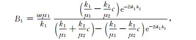
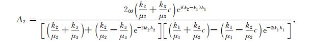
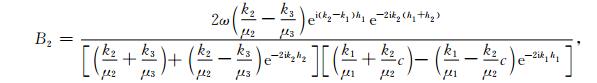
Appendix
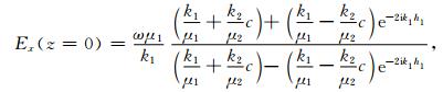
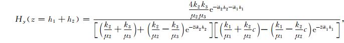
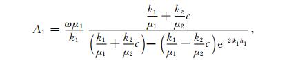
Electric and magnetic fields (E and H), and the impedance (Z=E/H) over and within a three layered half-space, at various depths z, at a circular frequency ω, as a resuit of an analytical derivation. The model parameters (electrical conductivity, magnetic permeability, thickness) are σj, μj, hj(j=1, 2, 3), and the complex wave number, 
At the surface:
|
(A1) |
|
(A2) |
where

|
(A3) |

|
(A4) |
At the boundary between layers 1 and 2:
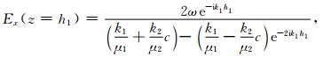
|
(A5) |
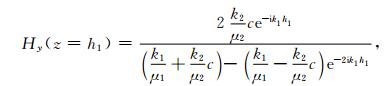
|
(A6) |
|
(A7) |
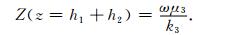
At the boundary of layers 2 and 3:

|
(A8) |
|
(A9) |
|
(A10) |
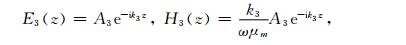
Within the individual layers

|
(A11) |

|
(A12) |
|
(A13) |
where
|
(A14) |
|
(A15) |
|
(A16) |
|
(A17) |

|
(A18) |
OTKA (Hungarian Scientific Research Fund) project number 68475.
| [1] | Hopkinson J. Magnetic and other physical properties of iron at a high temperature. Philosophical Transactions of the Royal Society of London, 1889, A, 180: 443-465. |
| [2] | Cracknell A P, Lorenc J, Przystawa J A. Landau's theory of second-order phase transitions and its application to ferromagnetism. J.Phys.C:Solid State Phys, 1976, 9: 1731-1758. DOI:10.1088/0022-3719/9/9/015 |
| [3] | Kiss J, Szarka L, Prácser E. Second-order magnetic phase transition in the Earth. Geophysical Research Letters, 2005, 32: L24310. DOI:10.1029/2005GL024199 |
| [4] | Rüdt C, Poulopoulos P, Babersche K, et al. Curie temperature and critical exponent g in a Fe2/V5 superlattice. SCM 2001, Physical Status Solidi (a), 2002, 189: 362. |
| [5] | Dunlop D J, Özdemir Ö.Magnetizations of rocks and minerals.In:Schubert G ed.Treatise on Geophysics.Volume 5.Geomagnetism.Elsevier, 2007 |
| [6] | Petrovský E, Kapiĉka A. On determination of the Curie point from thermomagnetic curves. J.Geophys.Res., 2006, 111: B12S27. |
| [7] | Radhakrisnamurty C, Likhite S D. Hopkinson effect, block-ing temperature and Curie point in basalts. Earth and Planetary Science Letters, 1970, 7: 389-396. DOI:10.1016/0012-821X(70)90080-4 |
| [8] | Kontny A, de Wall H. The use of low and high k (T)-curves for the characterization of magneto-minerological changes during metamorphism. Phys.Chem.Earth, 2000, 25: 421-429. DOI:10.1016/S1464-1895(00)00066-1 |
| [9] | Fowler C M R. The Solid Earth:An Introduction to Global Geophysics. New York: Cambridge University Press, 2005. |
| [10] | Kiss J.Gravity and magnetic data processing and modelling to improve our knowledge about the geo-environment[Ph.D.thesis].Sopron:University of West-Hungary, 2009 |
| [11] | Cao J, Li X, He Z. MT inversion including magnetic parameter.6th China International Geo-electromagnetic workshop. Extended Abstracts, 2004: 5-8. |
| [12] | Prácser E.Parametrization to geophysical inversion along profiles[Ph.D.thesis].Miskolc:Miskolc University, 2006 |
| [13] | Franke A, Boerner R U, Spitzer K. Three-dimensional finite-element simulation of electromagnetic fields using unstructured grids. 18th EMIW, 2006: S3-13. |
| [14] | Rijo L."Magnetic Statics" shift effects on 2-D TE magnetot-elluric sounding.In:8th International Congress of the Brasilian Geophysical Society.Rio de Janeiro, 2003, 1:1-6 |
| [15] | Szarka L, Franke A, Prácser E, Kiss J.Hypothetical mid-crustal models of second-order magnetic phase transition.4th International Symposium on Three-Dimensional Electromag-netics, Freiberg, Germany, September 27-30, 2007 |
| [16] | Ádám A, Szarka L, Steiner T. Magnetotelluric approxima-tions for the asthenospheric depth beneath the Békés Graben, Hungary. Journal of Geomagnetism and Geoelectricity, 1993, 45: 761-773. DOI:10.5636/jgg.45.761 |
| [17] | Ádám A. A search for the Hopkinson effect that is for a susceptibility enhancement at Curie depth in the Pannonia Basin. Magyar Geofizika (in Hungarian), 2008, 49(2): 68-74. |
| [18] | Jiles D.Introduction to Magnetism and Magnetic Materials.Boica Raton-London-New York:Taylor and Francis, 1998 |