 2010, Vol. 53


The Cenozoic Himalaya-Tibet orogeny is geo-dynamically active region to understand the crus-mantle structure, composition etc[1]. This is the reason for the ever increasing geophysical investigations such as seismic, electromagnetic etc., being conducted in this active collision zone to delineate the deeper structures and their possible relation with the ongoing deformation and processes. In recent years some Magnetotelluric (MT) measurements were made along profiles that cross parts of Southern Tibet and the Himalaya[2]. Although these profiles are distributed in eastern, central and western parts of Himalaya, their coverage in Himalaya-Tibet orogeny remain sparse due to logistic problems. A major gap lies in the Himalayan region between Vaikrita (MCVT) and Main Boundary Thrust (MBT). One of the important studies was INDEPTH[3] which deciphered deeper structure (up to 100 km) in the NE parts of Higher Himalayas, Indus Tsangpo Suture Zone to Southern Tibet. Some other MT studies to understand conductivity structure have also been undertaken on the NW[4?6], central7] and NE[3, 8] parts of the Himalayan region. Most of these MT experiments either cover the Higher Himalayas to Southern Tibet[3] or MBT to Siwalik/Dharmasala formations[5] except few studies[8, 9] which cover the zone between Higher Himalayas to south of MBT in the central part. It contains most of active thrust zones and epicenters of great earthquakes of Himalaya.
The North western Himalyan region is well known for its seismicity and falls within the VIII-X isoseismals of the 1905 great Kangra earth-quake[10, 11] where MCT/MBT take sudden northward turn. Because of this there is signiticant and very closely spaced assemblage of thrust belts between MCT and MBT. Keeping in view of the closely spaced thrust belts and noted seismicity during the past 110 m. y, MT investigations were carried out to derive the conductivity structure in the region from Higher Himalayas to Siwaliks.
2 Geology and tectonicsMajor domains of the Himalayan region (Fig. 1) are: (1) Higher Himalaya consists of amphibolite-grade schist and gneiss intruded by leuco-granitic plutons, which are bounded to the south by the Main Central Thrust (MCT) fault which roughly follows the belt front of the Higher Himalaya[12], (2) Lesser Himalaya forms the footwall of the MCT. It consists mainly of Precambrian to Paleozoic intensely deformed metasediments and is bounded to the south by the Main Boundary Thrust (MBT) [e. g., Gansser[13]] and (3) Sub-Himalaya, towards further south, consists of Tertiary molasses sequences involved in thin skinned tectonics induced by thrusting of the Himalaya over the Indian basement in the Siwalik Hills[13].

|
Fig. 1 Schematic crustal section of the Himalayan collision zone (Modified from Powers et al. [7]) |
It is considered that the major tectonic activity in the area takes place along the Main Himalayan Thrust (MHT), which reaches the surface along the Himalayan Frontal Fault (HFF), flattens beneath the Lesser Himalaya and roots along a ramp beneath the Higher Himalaya[14-17]. This fault appears to be connected with a major horizontal reflector under the Tibet as revealed by the INDEPTH CMP pro:file[18]. In the interseismic period, the MHT is locked from the surface until the base of the mid-crustal ramp, inducing stress build up and well clustered microseismic activity around the ramp[16, 19].
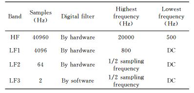
3 MT data acquisition, analysis and inversionThe MT measurements were made during May-July 2006 field season using a five-channel MT data acquisition system (ADU-06) of M/S Metronix, Germany. Three orthogonal magnetic fields (North-South, East-West and vertical) were measured at each sounding location along with two horizontal (North-South and East-West) electric field components. The magnetic field variations are measured using induction coils and electric field variations are measured using Cd/Cd-Cl2 nonpolarized electrodes. MT time series were recorded for 2~3 days in different frequency bands as shown in Table 1. Magnetotelluric data has been acquired at 16 sounding locations along a 150 km long profile extending from the Siwaliks in the south to the Higher Himalaya in the north (Fig. 2). The MT profile with N20°E direction and approximately perpendicular to the regional geological strike cuts across various geological and tectonic units. Interestingly in the southern part the profile cuts a cluster of thrusts viz. Palampur, MBT, Chail, Jutogh etc. as shown in Fig. 3.

|
Fig. 2 Geological map of the study area shown along with the MT sounding locations (shown by red symbols) |

|
Fig. 3 Southern part of MT profile cuts across the series of combined frontal and oblique thrust ramps |
|
|
Table 1 Different frequency bands under which MT data has been acquired using ADU-06 (after Friedrichs, 2003[20]) |
The measured MT time-series from the individual sites are visually inspected for noisy segments, such as spikes. The time-series obtained after the elimination of noisy segments are processed using robust algorithms included in the Mapros sottware[20] to estimate the MT impedances and the vertical magnetic field transfer functions as a function of frequency. The estimated MT impedances in general show good quality. Sounding data at two representative locations along the profile are illustrated in Fig. 4 as apparent resistivity and phase curves. To interpret these MT data quantitatively, t is necessary to convert frequencies to depths. Interpretation of MT data is routinely made from 2-D resistivity models derived from inversion of impedance values using 2-D inversion algorithm[21]. The application of 2-D algorithm requires a valid 2D approximation and geoelectric strike.

|
Fig. 4 MT data measured at two sounding locations (01 & 07) shown as apparent resistivity and phase curves The continuous line represents the smooth variation of data points. |
The impedance tensors for all stations at all frequencies were decomposed using the tensor decomposition procedure[22]. The unconstrained decomposition at different frequencies indicated that the shear had a stable value at most frequencies. The shear was then fixed to is average value and the decomposition procedure was repeated with unconstrained twist and strike angles. This resulted in a marked improvement in the stability of the twist and the strike angles. The twist was varied in the vicinity of is average value to further decrease the frequency dependence of the observed strike angles. The strike angles at different frequency bands are shown in the form of rose diagram (Fig. 5). The regional strike direction has been assumed to be either N50°E or perpendicular to it (i. e. N40°W). Most of the tectonic and geological features in the study area are aligned in NW-SE direction. Hence it is reasonable to assume a geoelectric strike direction of N40°W that comply with the geological trend in the area. Accordingly the data in measured direction has been rotated to N40°W.

|
Fig. 5 Rose diagram showing the geoelectric strike directions estimated using Groom-Bailey decomposition procedure |
To interpret the MT data, the next step is to take the MT data that is a function of frequency and convert it into a model of subsurface resistivity as a function of true depth. Two-dimensional (2D) resistivity models are generated through systematic 2D inversions of the regional MT impedances after projecting the MT sites onto a line perpendicular to the determined strike direction. The 2 D NLCG inversion algorithm of Rodi and Mackie[21] s used in this study. The NLCG algorithm uses non-linear conjugate gradients and s a stable algorithm that is widely used by both industry and academicians. This inverse problem is non-unique[23] and it can be shown that f a solution can be found, then an infinite set of models can also be found. Thus the inversion of MT data requires additional constraints for resistivity model to give a unique solution. A starting resistivity model was developed with a 100 Ωm half space.
The TE (transverse electric) and TM (transverse magnetic) mode data are initially inverted independently, for different combinations of error floors assigned to apparent resistivity and phase, to evaluate the suitable error floors required to produce acceptable misfit errors. This exercise enabled to verify the internal consistency between apparent resistivity and phase values at each sites and helped to identify the outliers (points showed large misfit), which are subsequently removed. The study suggested a minimum error floor of 20% in apparent resistivity and 5 % in phase required to fit the data within an acceptable r. m. s. error between the observed and computed responses. The inversion exercise continued with the joint inversion of the TE and TM data with error floors that are found to be suitable from the previous single mode inversions. The higher error floor set in the apparent resistivity (compared to the phase) data would help to overcome the possible static shift effects in the data. The data in the 0.01~400 sec period range is only inverted to construct the subsurface model.
In the algorithm the regularization parameter τ plays a significant role, controlling the balance between data fit and model roughness. A high value of τ produces a resistivity model that has a poorer fit to the measured MT data, but is spatially smooth. A small value of τ will give a better fit to the MT data, but the model may be rough and contain artifacts. In order to find an appropriate τ, the inversion studies are carried out several times with different τ values, i. e., 0.1, 0.3, 1, 3, 5, 10, 30, 100, 300. When the resulting r. m. s. errors are plotted against roughness, a typical L-shaped curve[24] is resulted and the preferable τ value lies in the knee of the L-curve. The L-curve plotted for the data set under study (Fig. 6) suggested a value of 3 for the roughness parameter. The other parameter that controls the inversion model is α which provides a balance between horizontal and vertical smoothness in the resistivity model. In general, a value of α greater than 1 results in a model with horizontal layering, while values of a below 1 produces vertical features. Inversion of MT data for different values of α(=0.3, 1 and 3) was undertaken and a value of α=1 found appropriate for this particular data set.

|
Fig. 6 L-curve generated for the present data set |
The different inversion models are generated using various combinations of inversion settings, such as single mode and joint inversion of TE + TM data. It is found that the joint models produced higher misfit value due to the difficulty in fitting TE-mode data during inversion. This may be due to the distortion effects, which could be more pronounced in TE mode impedances. It can be noted that the study area comprises severe topographic variations (400~4000 m) and hence appropriate to consider their effects during 2D modeling. To overcome these issues, TM mode inversion models were preferred, as this component of the MT impedance tensor is least affected by 3D induction effects. Topography is included as a part of the inversion to accommodate the possible effects due to large topographical changes along the profile. To generate robust resistivity models, the vertical magnetic field data (Hz) was also used in the inversion. An absolute error value of 0. 05 is assigned to the tipper data and the inversions are repeated for different combinations of inversion settings. This joint model (TM+ Hz) resulted consistent model features with different inversion settings. All the inversions assumed an initial haf-space model of 100 Ωm resistivity. The final model (Figs. 7 and 8) used for the interpretation is obtained after 200 iterations, from the joint inversion of both TM impedance data and tipper impedance along the strike. A wide range of permutations of inversion control and regularization parameters was investigated to ensure that the final resistivity model is robust (i. e. t does not depend on a particular choice of control parameters). The measured and computed MT responses are shown in Fig. 9 as apparent resistivity and phase pseudo sections. Note that the observed and computed data show reasonably good match indicating that the obtained MT model response fits well with the measured data. The statistical fit of the data can be measured by the root-mean-square (r. m. s.) misfit. A statistically ideal fit would be unity, but a value in the range 1~2 is generally considered acceptable. The present model (Figs. 7 & 8) has an r. m. s. misfit of 1.814 after 200 inversion iterations. The r. m. s. errors at individual sites are also presented in Fig. 10. The resistivity structure in the area resulted from the 2D inversion in the MT model is discussed in the following lines.

|
Fig. 9 Observed and computed (a) TM-mode responses and (b) Hz data are presented in pseudosection format for the Bilaspur-Rohtangpass profile MT data Station locations are denoted by the inverted triangles and the vertical frequency scale is logarithmic. |

|
Fig. 10 Plot showing the variation of r.m.s. error along the MT profile |
The modeling of MT data along the 150 km long N-S oriented Bilaspur-Rohtangpass profile as shown in Fig. 7 (Shallow) and Fig. 8 (Deep) bring out certain distinct features of different resistivities A~F. These are described below along with the possible geological and tectonic features which might have contributed to the significant resistivity variations observed beneath this profile (Fig. 2).

|
Fig. 7 The shallow section of the resistivity model obtained from the joint inversion of TM impedance data and Hz data using NLCG inversion scheme Dashed lines indicate the approximate boundary between different resistive/conductive layers. The northward dipping nature of the marked layers corresponds to the geological formations of the subducting Indian plate. |

|
Fig. 8 The deep resistivity model obtained from the joint inversion of TM impedance data and Hz data using NLCG inversion scheme Dashed lines indicate the approximate boundary between different resistive/conductive layers. The northward dipping nature of the marked layers corresponds to the geological formations of the subducting Indian plate. The model illustrates a near vertical conductive (~10 Ωm) feature (B) extending to deep crustal levels, spatially coincides with the MBT. Also, high resistive (>1000 Ωm) block (G) underneath the Rampur window s also mapped n MT model. |
Feature-A: This s a shallow (extending up to -8 km depth) conductive (2~16 Ωm) feature which lies near the southern end of the profile G. e. south of MT station No. 16), as shown in Fig. 7. This high conductive layer seems to be indicative of the presence of the Siwalik/Dharmasala group of sediments[17].
Feature-B: This feature seems to be a deep penetrating (>40 km) and nearly vertical conductive anomaly (~10 Ωm). Interestingly it coincides spatially with the Main Boundary Thrust (MBT) of the Himalayas and closely associated with other thrusts/faults[25, 26] as shown in Fig. 8. It may be noted that this feature lies close to the Kangra reentrant of the Himalayan tectonics, wherein the MBT characterized by the feature B takes a northern and then westward turn (see Fig. 2) and then passes through very close vicinity of the epicenter of the Great Kangra earthquake. The close proximity of the Rampur window[27] of the Lesser Himalaya on the eastern side of the Chail thrust region and the basement ridges[28, 29] on the western side of the Chail thrust region would have contributed to the northward turn of these (otherwise NW-SE oriented) thrust belts (Kangra reentrant). It is possible that the fluid content of the MBT continues from the MT station No. 16 to Kangra region.
Feature-C: It represents a northward dipping conductive zone (5~30 Ωm) which could be due to the Shali-Deoban group of sediments plus the luid content of the Chail thrust (Fig. 7) in Lesser Hima-kyan region. It may be noted that the MT profile, here, runs along the Chail (Panjal) thrust.
Feature-D: A high resistive (> 5000 Ωm) north dipping block revealed between Chail and Jutogh (Munsiati) thrusts containing Chail metamorphics and may correspond to the overthrusting of the crystalline basement[15] as shown in Fig. 7.
Feature-E: This is a low angle north dipping conductive zone (~50 km) lyingbetween J (M) T and MC (V) T. Fluid content in this zone seems to have contributed to this conductive anomaly. This s supported by the sequence of hot springs on the surface shown by red symbols in the Fig. 7.
Feature-F: A near surface highly resistive (>5000 Ωm) zone most probably represents the Higher Himalayan crystallines.
Feature-G: It represents a deeply buried (>8 km) and highly resistive (>2000 Ωm) and near vertical zone (Fig. 8) of the Lesser Himalayan crystallines under the well known ‘Rampur window'[27]. The confined nature of this buried (8~50 km) resistive body is reflected on the surface in the form of elliptical shaped' Rampur window' (Fig. 2).
Integration of these models with other geophysical data sets like gravity, seismic tomography etc. is under progress and may throw further light on the issues.
The study re-emphasizes the utility of the MT investigations in the tectonically active Himalaya-Tibet orogeny. The reason for the efficacy of this method appears to be the conductivity (or resistivity) contrasts that one may expect at the interface of sediments (often wet and/or moist) and/or fluids, and the basement. In spite of this, the MT studies in this region have been a few, indicating there is a great need of imaging the electrical structure of the crust and mantle beneath the Himalaya-Tibet orogeny, especially to monitor the earthquake prone regions. In this connection it s pertinent to note that the present profile falls well within the VIII-X isoseismal[10] of the Great Himalayan earthquake of 1905 with its epicenter being near Kangra.
AcknowledgementsWe thank Dr V. P. Dimti, the Director of NGRI for constant encouragement and support. We express our gratitude to Dr Upendra Raval for his valuable suggestions and discussions during the study. The critical comments/suggestions from Prof A. Adam and the other anonymous reviewer have greatly improved the manuscript. MT data collection and analysis was made possible with funding support from Ministry of Non-conventional Renewable Energy, New Delhi.
| [1] | Valdiya K S. Geology of Kumaun Lesser Himalaya. Wadia Institute of Himalayan Geology, Dehra Dun, India, 1980 Valdiya K S. Geology of Kumaun Lesser Himalaya. Wadia Institute of Himalayan Geology, Dehra Dun, India, 1980 |
| [2] | Unsworth M J, Jones A G, Wei W, et al. Crustal rheology of the Himalaya and Southern Tibet inferred from magnetotelluric data. Nature, 2005, 438: 78-81. DOI:10.1038/nature04154 |
| [3] | Spratt J E, Jones A G, Nelson K D, et al. Crustal structure of the India-Asia collision zone, southern Tibet, from INDEPTH MT investigations. Physics of Lhe Earth and Planet. Inter., 2005, 150: 227-237. DOI:10.1016/j.pepi.2004.08.035 |
| [4] | Gokarn S G, Gupta G, RaoC K, et al. Electrical structure across the Indus Tsangpo suture and Shyok syture zones in NW Himalaya using magnetotelluric studies. Geophy. Res. Lett., 2002, 29: 1251. |
| [5] | Gokarn S G, Rao C K, et al. Crustal structure in the Siwalik Himalayas using magnetotelluric studies. Earth Planets Space, 2002, 54: 19-30. DOI:10.1186/BF03352418 |
| [6] | Arora B R, Unsworth M J, Rawat G. Deep resistivity structure of the northwest Indian Himalaya and its tectonic implications. Geophy. Res. Leu., 2007, 34: L04307. |
| [7] | Pham V N, Boyer D, Therme P, et al. Partial melting zones in the crust in southern Tibet from magnetotelluric results. Nrue, 1986, 319: 310-314. |
| [8] | Patro B P K, Harinarayana T. Deep geoelectric structure of the Sikkim Himalayas (NE India) using magnetotelluric studies. Physics of he Earth and Plane. Inter., 2009, 173: 171-176. DOI:10.1016/j.pepi.2008.10.011 |
| [9] | Lemonnier C, Marquis G, Perrier F, et al. Gophy. Rc. Lee, 1999, 26: 3261-3264. |
| [10] | ThakurV C, Sriram V, Mundepi A K. Seismotectonics of the great 1905 Kangra earthquake meizoseismal region in Kangra-Chamba, NW Himalaya. TecLono physics, 2000, 326: 289-298. |
| [11] | Gupta H K. Major and great earthquakes in the Himalayan region: an overview. In: Gupta H K ed. Disaster Management. Universities Press (India) Private Limited, India, 2003 Gupta H K. Major and great earthquakes in the Himalayan region: an overview. In: Gupta H K ed. Disaster Management. Universities Press (India) Private Limited, India, 2003 |
| [12] | Le Fort P. Himalayas:the collided range, present knowledge of the continental arc. A. J. of Sci., 1975, 275: 1-44. DOI:10.2475/ajs.275.1.1 |
| [13] | Gansser A. Geology of the Himalayas. New York: Interscience Publ., 1964. |
| [14] | Molnar P. Inversion of profiles of uplift rates for the geometry of dip-slip faults at depth, with examples from the Alps and the Himalaya. Ann. Geophysicae, 1987, 5: 663-670. |
| [15] | Schelling D, Arita K. Thrust tectonics, crustal shortening and structure of the.ar-eastern. Nepal Himalaya. Tectonics, 1991, 10: 851-862. DOI:10.1029/91TC01011 |
| [16] | Pandey M R, Tandukar R P, Avouac J P, et al. Gophy. Rc. Lee, 1995, 22: 751-754. |
| [17] | Powers P M, Lillie R J, Yeats R S. Structure and shortening of the Kangra and Dehra Dun reentrants, Sub-Himalaya, India. GSA Bulletin, 1998, 110: 10101027. |
| [18] | Zhao W, Nelson K D. Project INDEPTH Team Deep seismic reflection evidence for continental underthrusting beneath southern Tibet. Nuwre, 1993, 366: 557-559. |
| [19] | Bilham R, Larson K, Freymuller J, et al. Indo-Asian convergence rates in the Nepal Himalaya. Nature, 1997, 386: 61-66. DOI:10.1038/386061a0 |
| [20] | Friedrichs B. MAPROS-ADU Data Acquisition and Processing Manual 2003 Friedrichs B. MAPROS-ADU Data Acquisition and Processing Manual 2003 |
| [21] | Rodi W, Mackie R L. Nonlinear conjugate gradients algorithm for 2-D magnetotelluric inversion. Geophysics, 2001, 66: 174-187. DOI:10.1190/1.1444893 |
| [22] | Groom R W, Bailey R C. Decomposition of the magnetotelluric impedance tensor in the presence of local three dimensional galvanic distortions. J. Gophy. Rc., 1989, 94: 1913-1925. DOI:10.1029/JB094iB02p01913 |
| [23] | Parker R L. Geophysical Inverse Theory. Princeton University Press, 1994. |
| [24] | Hansen P C. Analysis of discrete ill-posed problems by means of theL-curve. SIAMRer., 1992, 34: 561-580. |
| [25] | Dubey A K, Bhakuni S S, Selokar A D. Structural evolution of the Kangra recess, Himachal Himalaya:a model based on magnetic and petrofabric strains. J. Asian Earth Sci., 2004, 24: 245-258. DOI:10.1016/j.jseaes.2003.11.002 |
| [26] | Pandey A K, Sachan H K, Virdi N S. Exhumation history of a shear zone constrained by microstructural and fluid inclusion techniques:an example from the Satluj valley, NW Himalaya, India. J. As'an EaUhSs, 2004, 23: 391-406. |
| [27] | Pandey A K, VirdiNS N S, GairolaVK V K. Evolution of structural fabrics and deformation events in the Kulu-Rampur and Larii windowzones, NW Himalaya, India. Himalayan Geology, 2003, 24(1): 1-21. |
| [28] | Raiverman V, Kunte S V, Mukherjee A. Basin geometry, Cenozoic sedimentation and hydrocarbon prospects in north western Himalaya and Indo-Gangetic plains. In: Bhandari L L eds. Petroliferous Basins of India. Petroleum Asia Journal, 1983, 6:67-92 Raiverman V, Kunte S V, Mukherjee A. Basin geometry, Cenozoic sedimentation and hydrocarbon prospects in north western Himalaya and Indo-Gangetic plains. In: Bhandari L L eds. Petroliferous Basins of India. Petroleum Asia Journal, 1983, 6:67-92 |
| [29] | Raval U. Collision boundary, stress build-up and role of basement heterogeneities:a peg effect. Proceedings if the IGU Annual Seminar on 4 Geophysics for Runl Development', 1993: 129-140. |