 2010, Vol. 53


 , LIU Jing1, SHEN Xu-Hui1, M.Parrot 2, QIAN Jia-Dong1, OUYANG Xin-Yan1, ZHAO Shu-Fan1, HUANG Jian-Ping1
2. LPC2 E/CNRS, 3A Avenue de la Recherche Scientifique, 45071 Orléans cedex 2, France
2. LPC2E/CNRS, 3A Avenue de la Recherche Scientifique, 45071 Orléans cedex 2, France
DEMETER, a French micro satellite, was the first one in the world to be designed specially for studying the ionospheric variation possibly associated with earthquakes, having a solar synchronous circular orbit, declination of 98. 23°, and height of 710 km (which decreased to 660 km in mid December 2005). A lot of strong earthquakes have occurred since it was launched on 29 June 2004. The Sumatra earthquake sequence was one of them, starting from the main M 9.3 shock in the region of Sumatra, Indonesia, on 26 December 2004. Some papers have dealt with ionospheric variations associated with this sequence by using data from the DEMETER mission centre. [1~3]
Among these studies, great interest was placed on the features of spatial distribution of the ionospheric parameters along the latitude and its temporal evolution, showing the so-called equatorial anomaly in the parameter of electron density, with a deep valley-like trough near the magnetic equator and two peak-like crests distributed at latitudes of about 20° north and south respectively. The equatorial anomaly is a regular phenomenon in the F2 layer of the ionosphere. and is sensitive to the variations in the seismo-generated vertical electric field around the equatorial area[1, 4, 5]. In contrast to the crests, the trough of a day, if it is in quiet magnetic conditions, would appear in the early morning, reach its greatest development in the afternoon, and then gradually degrade with both crests moving towards the equator from the north and the south respectively until a single peak occurs near the equator at night[4, 5, 1]. It was reported[1] that equatorial anomalies had been registered in GPS TEC (Total Eleetron Content) since 21 December, five days prior to the main shock of the Sumatra earthquake sequence, and became most developed in the evening and night-time of 25 December, which would be the time showing a single peak near the magnetic equator in the latitudinal distribution of electron density as mentioned above.
This paper deals with the behaviors related to the latitudinal distribution of electron density associated with the case of an earthquake from the sequence which was the biggest aftershock, with a magnitude of 8. 6, a depth of about 3O km, and epicentre coordinates of 2. 09° N and 97. 11° E, occurring at 20 : 05 on 28 March, about which Pulinets et al. presented their results at the international symposium DEMETER, 14~16 June, Toulouse, France, with a few orbits on 22 March near the epicentre being chosen to show this equatorial variation feature. In this paper, however, more data have been taken into account, so that some new results are available for further discussion on the anomaly.
2 DataThe data were taken from orbits when the satellite was flying over the epicentral area and its neighborhood and were downloaded from the DEMETER mission centre between 1 March and 5 April, a period of more than one month that covered the date of the earthquake occurrence in this case.
Among the data only those from half up-orbits (in which the satellite passed over the studied region during the local nighttime around 22: 00) could be used in this paper, due to the fact that the ionospheric environment of half down-orbits is strongly affected by the regular solar radiation in the local daytime.
Also, the data for those dates with strong solar activities denoted by geomagnetic indexes Kp exceeding 4 were removed from the data coverage in this paper in order to verify whether or not some anomalous variations in the ionospheric parameters possibly associated with the studied earthquake case could be found. As shown in Fig. 1, such an ionospheric environmental condition appeared for almost half of the month of March 2005.

|
Fig. 1 Geomagnetic condition the Kp index histogram (a) and the Dst index curve during March 2005 |
In order to consider information for the study of the earthquake cases, methodology concerning the term "anomaly" must be recognized. The synchronous variations could be supposed to be an anomaly if they appear in parameters of two or more kinds in some segments on the studied orbit.
Comparing all the orbits over the region within a distance of 2000 km apart from the epicentre area, from the database left after the data selection mentioned in the last section. it is found that only on 22 and 23 March (see Fig. 2) did obvious anomalies occur in the equatorial region that are largely different from those on other days, with at least six kinds of parameters showing synchronous variations, as shown in Fig. 2 from the top to the bottom panels respectively, which are the following: the electron density (Ne), the electron temperature (Te), the ion densities of O+, H+, and He+, the ion temperature (Ti), the spectrum of the VLF electric field, and the spectrum of the VLF magnetic field. Except for the spectrum of the VLF magnetic field, significant perturbations are exhibited in a range from 20° S to 20° N among these parameters.

|
Fig. 2 Disturbed orbits on 22 (A) and 23 (B) March above the epicentral area |
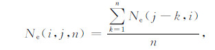
All half up-orbits (in LT nighttime) passing over the region within 2000 km from the epicentre were picked up, and data for electron density (Ne) in the latitude range between 20° S and 20° N in each orbit were taken in order to construct a kind of time sequence for the selected parameter and to compare the variations above the earthquake region and in the equatorial area on different dates. It is known that two crests in the equatorial ionization anomaly (EIA) are usually located at+/-10~15° N geomagnetic latitude respectively. This means that the region of crests appearance is inside the region of 20° S~20° N that we selected for studying. According to the satellite orbit design (solar synchronous with a height of 710 km), the time period for a satellite flying over the latitude range from 20° S~20° N is supposed to be a little shorter than 20 minutes, with approximately the same local time for each studied orbit. The special time sequence was constructed in the following steps. Firstly, an orbit sequence was formed from the selected ones and arranged based on the orbit number list from the smallest to the largest. Secondly the average obtained by analysis of the data for each given point of the segment over the latitude range of 20° S~20° N by its former five or ten orbits, was taken as the value of the given point in the last orbit, and an averaging time sequence for the segment of the orbit was formed. The processing can be explained by Formula (1).
|
(1) |
where i represents the given latitudinal point varying from -20° S to 20° N of the jth orbit, and Ne(i, j, n) represents the computation value of electron density at theithpoint of the jth orbit averaged over its former n orbits, that is the averaged time sequence of electron density in the given segment of the jth orbit. As mentioned above, here n=5 or 10; however n could be any number as preferred. Thirdly, those averages are taken for each orbit and each averaged time sequence is connected based on the orbit list number to construct the special time sequence as shown by the blue line in Fig. 3. The same steps can be applied to carry out deviation analysis to construct two special time sequences with±lσ deviated from the mean value respectively: one is called the upper-limk one and the other the lower-limtt one, as shown by the red and pink lines in Fig. 3, and both have the same feature as the averaged one. As for every value at its corresponding latitude, 5 or 10 values at the same latitude recorded on its former orbits were averaged to obtain the mean value. So the comparison was made only among the values at the same latitude to avoid the spatial effects at different latitudes. This means that if an anomaly occurred, this value was much smaller or larger than the limits at the same latitude of its former 5 or 10 orbits. Five orbits were selected to be the averaged window, due to the similarity among different orbits during a relatively short time period. Ten orbits were considered for the averaged window here because in M arch 2005 there were too many disturbed days being involved, so that a smooth picture would be available.

|
Fig. 3 Ne curves from 20 March to 5 April above the epicentral area (a)5 orbits sliding averaged line and its limited lines; (b)10 orbits sliding averaged line and its limited lines. |
All these curves are shown as temporal series with a small cut between two orbits (Fig. 3a and 3b) since 20 M arch, the relatively quiet magnetic activity in this month. In Fig. 3, the x-axis is labeled by orbit number and its date of observation. It is shown that on the same distance scale, sometimes only one half orbit was found and sometimes two half orbits were found on the same day. It can be seen that the averaged line of five orbits varied significantly between different orbits (Fig. 3a), while the 10 averaged lines were similar with relatively steady amplitudes (Fig. 3b). But in these two figures, three orbits exceeded the upper line significantly in the same way on 20, 25, and 28 M arch respectively. Based on the public data about quiet days and most disturbed days from the GFZ German Research Centre for Geosciences (http://gfz-potsdam.de), the increasing Ne on 20 and 28 March might be caused by other sources possibly associated with the preparation process of Sumatra 8. 6 earthquake. Especially, the orbit recorded on 28 March flew just over the epicentre area about 30 minutes before the earth-quake occurrence, reflecting the imminent intense perturbations in the ionosphere just before this event.
In addition. it is worth noting in Fig. 3 that the perturbations of the orbits of 3827 and 3842 recorded on 22 and 23 March in 2005 were different from other curves, with changes exceeding not only the upper limit but also the lower limit. On the basis of the analysis mentioned above, four anomalies orbits at local nighttime on 20, 22, 23, and 28 March were detected in quiet magnetic condition. Due to the fact of diurnal solar activity, the variations in N at 20° S~20° N for most orbits in Fig. 3, show a single peak just near the equator that represents the typical shape of Ne at 710 km altitude. except for the variations on 22 and 23 with double crests and deep troughs in the equatorial area, which would be taken as a peculiar behaviors. It seems to the authors that the feature would be similar to the one described in the research on anomalous variations for GPS TEC Drior to 2004 Indonesian M 9.0 earthquake on Dec. 26 by Zakharenkova et al[1]. Eli, in which the modification of the equatorial anomaly occurred a few days prior to the earthquake, and except for the daytime amplification of the Appleton anomaly, the meridian section of TEC spatial structure took the shape of a double-crest curve with a trough near the epicenter. So the occurrence of this phenomenon at these orbits demonstrates intensive ionospheric perturbations on those two days, which may be related to this Sumatra M 8. 5 earthquake. Also, Ouzonov et al.[11] showed that GPS TEC was observed to increase on four days (March 22~25, 2005) prior to the event with low Dst values. In their study of TEC anomalies related to the earthquake swarms during the time period of Dec 2004~Apr 2005, the anomaly appeared not to be atmospheric effects due to its long persistence over the same region.
3.2 GIobal featureIn order to reflect the global feature of Ne anomalies on M arch 20, 22, 23, 28 before the Sumatra M 8. 6 earthquake, the data for all the orbits around the world recorded at local nighttime were selected for M arch 20, 22 and 28 in 2005 for comparison (Fig. 4), and the data for 4 March in the quiet time were chosen as the normal background variation for the purpose of comparison. This showed that on 4 M arch, Ne exhibited a single peak at the equatorial area in all orbits, which was also the seasonal feature in the local nighttime[12]. On 20 March, the spatial shape of electron density was consistent above the whole globe, with a single peak of electron density Ne occurring in the equatoriaI area in the scale of 0~20° N at O~200° E and 0~1O°N at 200~360°E, which corresponds to the magnetic equator of the east and west half globes. However it is remarkable that the peak values on 20 March were mostly larger, with amplitudes above 50000 cm-3, than those on 4 March, which had amplitudes mostly lower than 40000 cm -3. That is to say, the increasing amplitude on 20 March in most orbits was much greater than that on 4 March. March 4 and 20, 2005 are both during the quietest magnetic time, and the orbits are revisited in a period of 16 days. So it can be concluded that the anomalies on 20 March disturbed almost the whole ionosphere and were not regional anomalies. Comparing the picture of Ne on 20 March with the peak regions and amplitude of Ne on 22 March, they are seen to be similar. However on 20 March there s increasing variation only in the equatorial area, while on 22 March, decreasing variation among the peak values occurred, forming apparent troughs in this area. The anomaly feature which s the same on March 20 and 22 in 2005 is that they are all distributed above most of the globe and not just around the epicentral area. The difference between them is that on 22 March, Ne showed double crests, which is to say that the mechanism of perturbations on 22 March may be different from that on 20 March, and even resulted in the change from a normal single peak shape at the equator to double ones. On March 28, 2005, the picture s similar with that on March 4, with single peak values occurring at the equatorial area. But there s only one orbt nearest to the epicenter (Fig. 4) showing peak values exceeding 50000/cm-3. That is to say, the anomalies on March 20 and 22, 2005 distributed in a global scale, but on the day when earthquake took place, there was only the nearest orbt observing anomalies, showing much local feature.

|
Fig. 4 Ne distribution on March4, 20, 22 and 28 in 2005 |
Accompanying the variation of Ne on March 22 and 23, 2005, low frequency perturbations in theVLFelectric field occurred simultaneously (see Fig. 2). These perturbations of the VLF electric field were selected and are plotted in Fig. 5 for the total data recorded on 22 March. To allow a convenient comparison and visualized figures, electric field perturbations continuous above 100 μV2·m-2 ·Hz-1 just at the low frequency part from 19. 5~200 Hz according to Fig. 2 were chosen and assigned values of 1, and those data lower than 100 μV2·m-2 ·Hz-1 were assigned values of 0. So all the perturbations along the orbits at the low frequency part could be found, and the results are plotted in Fig. 5. In order to study whether these anomalies showed a conjugated feature, the geomagnetic coordinate is used in Fig. 5. It shows that the low frequency electric field perturbations near the magnetic equator on 22 March mainly occurred on seven orbits, of which six orbits were in the longitudinal scale of 100° and latitudinal scale of 30° to the epicentre, which presenteda smaller anomalous area than that of Ne. Although the perturbations all occurred at two positions on each orbit, neither was at the magnetic conjugate point of the other. Therefore, these anomalies may not be the equatorialfountain efect in the ionosphere referred to in the introduction, or they may have been affected by other factors.

|
Fig. 5 VLF electric field perturbations (black points) on 22 and 28 March 2005 |
As for the variations on 20 and 28 March with only monotonously increasing Ne, after the same data processing mentioned above, the electric field perturbations were presented only at the nearest orbtt to the epicentre, of which the image of 28 March s shown in Fig. 5.
Relative to the Ne global variations, the anomalous area of the electric field was obviously smaller and much more concentrated above the epicentral area, as on 28 March, which reflects the correlation between the ionospheric electric field anomaly and earthquake preparation zone, and electric signals have a much more local feature relative to Ne before this case.
4 Discussion and ConclusionIncreasing Ne and electrostatic turbulence have occurred under many conditions, sometimes during periods of geomagnetic storm, sometimes around strong earthquake occurrences. Are there any differences or does the same feature exists in these anomalous examples?
Berthelier et al. [6] introduced the instrument of ICE payload on DEMETER. In their paper, an example of electrostatic turbulence at the equator was exhibited on 16 September 2004 (Fig. 6), which was during disturbed days. The perturbations also occurred in every parameter, such as electric field, Ne, Ni(O+, H+, He+), Ti, , and so on, at the latitudinal scale of -1°~10°N in the Ne peak region. They thought that this anomaly originated from the satellite crossing plasma irregularities with a typical scale from a few metres to a few hundreds of metres. The ion density recorded by IAP displayed fast variations and was in an anti-correlation with the ion temperature. The electrostatic turbulence on 22 March 2005 was concentrated in two regions, which were different from that on 16 September 2004 (Fig. 6). Another large difference is shown the O+ density decreased, and the H+ density increased significantly, showing contrary variation on 22 March 2005, (see Figs. 2 and 6), while on 16 September 2004, H+ densitv varied with the same trend as that of O+ (Fig. 6). The comparison might illustrate the difference in mechanism for the two cases: the one controlled by the magnetic storm and the one by the earthquake preparation. Boskova et al.[13, 14] reported the phenomena of increased concentration of H+ and He+ recorded onboard the Intercosmos-24 satellite at an altitude between 2300~2500 km before the Iranian earthquake of 20 June 1990 with a magnitude of M s7. 7, located at 49. 409°E, 36. 957° N. Pulinets et al. [15]also studied the ion composition but at the lower altitude of the AE-C satellite. When the AE-C satellite passed over the earthquake preparation area, a decreased mean ion mass was observed, which is equivalent to an increase in the light ion concentration. All this evidence illustrates that the ionospheric perturbations in the ion composition due to earthquakes are different from those resulting from other geophysical factors. These phenomena provide a useful tool for us how to distinguish the anomalies resulting from earthquakes by combining the electric field and ion composition variations.

|
Fig. 6 Level-2 figures of a few parameters recorded onD EMETER respectively on 16 September 2004 (from Berthelier et al., 2006) and 22 March 2005 |
The equatorial anomaly reacts sensitively to all changes (of any origin) in electric fields. Prior to this Sumatra M 8. 5 earthquake, the electrostatic turbulences occurred accompanied by perturbations in plasma parameters in the equatorial area at DC-250Hz. They were distributed on a large scale of 100° longitude. In other studies, the Intercosmos-19 satellite also observed similar anomalous VLF emissions associated with the Irpinia earthquake[16, 17] in south Italy on 23 November 1980 (41. 30°E, 15. 52°N. M6. 9). In that case, the pre-earthquake effects were quite significant in size (2O~30° in latitude and 1 20° in longitude). The registered anomalous VLF emissions and effects in the conjugated area show that all of the magnetic tube was affected by the earthquake preparation process. The ionospheric anomalies before these two earthquakes are similar. But the Sumatra earthquake is located near the equator, where the magnetic lines of force are distributed horizontally, which makes it inconvenient for electromagnetic waves to penetrate into the ionosphere directly and reach its conjugate point as at relatively higher latitudes, especially for such low frequency electromagnetic signals.
In this paper. the local nighttime data were collected at a distance of 2000 km from the epicentre of the Sumatra M 8. 6 earthquake, in order to avoid the intense effects from the sun and other space factors. Based on the above analysis and discussion, some anomalies occurring in parameters such as the VLF electric field, electron density. electron temperature, ion density, and so on have been demonstrated. After comparison with other studies. it has been illustrated that these anomalies may be related to the Sumatra M8. 6 earthquake. Due to the larger intensity of this earthquake, the duration time of ionospheric anomalies prior to it was more than 1 2 hours and the affected area was larger than a hemisphere. The main conclusions drawn are as follows.
(1) The remarkable anomalies of Ne occurred 10 days before this earthquake, on 20, 22, 23, and 28 M arch respectively. On 20 and 28 March, the single peak in the equatorial area was maintained but the peak amplitudes on most orbits around the globe increased by over lσ relative to the normal peak values. As for the variation on March 22 and 23, 2005, the single peak shape of Ne above the equatorial area had changed to double crests with deep troughs occurring near the equator. The same characteristic of both kinds of anomalies appeared in a relative larger area, showing a global feature, except for the anomaly at nearest orbit to the epicenter on M arch 28, the day when Sumatra earthquake occurred.
(2) Low frequency electric field perturbations generally accompanied the Ne anomalies. With the single increasing Ne, there was only one group of electric field anomalies, but with double crests of Ne, two groups of electric field anomalies also formed. From the global distribution of low frequency electric field perturbations, the electric field anomalies occurred in the region above the epicentral area. Especially, when increasing Ne variation existed only in the equatorial area, the electric field anomalies occurred only on the orbit nearest to the epicentre. The two groups of Ne and elec: tric field anomalies in the orbits on March 22 and 23 in 2005 did not show the conjugate feature in the geomagnetic coordinate system. It is considered that it is difficult for the low frequency electric field to penetrate directly from the surface to the ionosphere due to the horizontal magnetic field in the equatorial area. So it might be reasonable that the electric field signals resulting from the seismic preparation processes may lead to the production of an acoustic-gravity wave in the atmosphere and may then disturb the ionosphere and lcad to other variations in plasma parameters and electric field[3, 18].
(3) Combined with other studies from different authors. the ion composition can be used as a tool to distinguish the effects from magnetic storms or earthquakes. In this paper, the density of different ions exhibited reverse varying shapes, which is consistent with those results before earthquakes. To determine whether the ionospheric anomalies were related to the earthquakes, conjoint analysis should be used on all kinds of parameters. besides considering the types of space indexes. The mechanisms of ion composition and variation with magnetic storms and earthquakes are complex, and further studjes should be carried out.
AcknowledgementsThis paper is funded by the National Science and Technology Support Project (2008BAC35B01, 2008BAC35B05). We are grateful to the DEMETER Data Centre of France for provi-sion of the satellite data.
| [1] | Zakharenkova I E, Krankowski A, Shagimuratov I I. Modification of the low-latitude ionosphere before the 26 December 2004 Indonesian earthquake. Nat.Hazards Earth Syst.Sci., 2006, 6: 817-823. DOI:10.5194/nhess-6-817-2006 |
| [2] | Parrot M, Statistical studies with satellite observations of seismogenic effects, in:Atmospheric and Ionospheric Elec-tromagnetic Phenomena Associated with Earthquakes, edited by:Hayakawa M, Terra Scientific Publishing Company, Tokyo, Japan, 1999, 685-695 |
| [3] | Pulinets S A, Boyarchuk K. Ionospheric Precursors of Earthquakes. Berlin: Springer, 2004. |
| [4] | Hanson W B, Moffett R J. Ionization report effects in the equatorial F region. J.Geophys.Res., 1966, 71: 5559-5572. DOI:10.1029/JZ071i023p05559 |
| [5] | Tsai H F, Liu J Y, Tsai W H, et al. Seasonal variations of the ionospheric total electron content in Asian equatorial anomaly regions. J.Geophys.Res., 2001, 106(A12): 30363-30369. DOI:10.1029/2001JA001107 |
| [6] | Berthelier J J, Godefroy M, Leblanc F, et al. ICE, the electric field experiment on DEMETER. Planetary and Space Science, 2006, 54: 456-471. DOI:10.1016/j.pss.2005.10.016 |
| [7] | Berthelier J J, Godefroy M, Leblanc F, et al. IAP, the thermal plasma analyzer on DEMETER. Planetary and Space Science, 2006, 54: 487-501. DOI:10.1016/j.pss.2005.10.018 |
| [8] | Lebreton J P, Stverak S, Travnicek P, et al. The ISL Langmuir Probe experiment and its data processing onboard DEMETER:scientific objectives, description and first results. Planetary and Space Science, 2006, 54: 472-486. DOI:10.1016/j.pss.2005.10.017 |
| [9] | Parrot M, Benoist D, Berthelier J J, et al.The magnetic field experiment IMSC and its data processing onboard DEMETER:scientific objectives, description and first results.Planetary and Space Science, 2006, 54:441-455 |
| [10] | Sauvaud J A, Moreau T, Maggiolo R, et al.High energy electron detection onboard DEMETER:the IDP spectro-meter, description and first results on the inner belt.Planetary and Space Science, 2006, 54:502-511 |
| [11] | Ouzounov D, Pulinets S, Ciraolo L, et al, Analysis of GPS Total Electron Content (TEC) and satellite electromagnetic data of atmospheric processes related to the northern Sumatra earthquake swarms of Dec 2004-Apr 2005, American Geophysical Union, fall meeting 2006, Abstract T34B-08 |
| [12] | Ouyang X Y, Zhang X.M., Shen X.H., et al. Study on ionospheric Ne disturbances before 2007 Pu'er, Yunnan of China, earthquake. Acta Seismologica Sinica, 2008, 21(4): 425-437. DOI:10.1007/s11589-008-0425-8 |
| [13] | Boskava J, Smilauer J, Jiricek F, et al. Is the ion composition of the outer ionosphere related to seismic activity? J. Atmos.Terr.Phys., 1993, 55: 1689-1695. DOI:10.1016/0021-9169(93)90173-V |
| [14] | Boskava J, Smilauer J, Triska P, et al. Anomalous behavior of plasma parameters as observed by the Intercosmos 24 satellite prior to the Iranian earthquake of 20 June 1990. Studia Geoph.Geod.(38): 213-220. |
| [15] | Pulinets S A, Legen'ka A D, Gaivoronskaya T V, et al. Main phenomenological features of ionospheric precursors of strong earthquakes. J.Atm.Solar Terr.Phys., 2003, 65: 1337-1347. DOI:10.1016/j.jastp.2003.07.011 |
| [16] | Ruzhin Y Y, Larkina V A.Magnetic conjugation and time coherency of seismo-ionosphere VLF bursts and energetic particles, in Proceedings of International Wroclaw Sympo-sium on Electromagnetic Compatibility, Wroclaw, 1996.645-648 |
| [17] | Ruzhin Y Y, Larkina V A, Depueva A K. Earthquake precursors in magnetically conjugated ionosphere regions. Adv.Space Res., 1998, 21: 525-528. DOI:10.1016/S0273-1177(97)00892-2 |
| [18] | Pulinets S A.Physical mechanism of the vertical electric field generation over active tectonic faults.Advances in Space Research, 44(6):767-773, 2009, doi:10.1016/j.asr.2009.04.038 |