The digital predistortion is a cost-effective way to the linearize power amplifiers. Memory polynomial is one of the most popular DPD models. However, these models cannot get a good compromise between accuracy and complexity. The author proposes a feedback-based model to characterize DPD. The model not only uses the input information, but also uses the past output information. Simulations show that the model can linearize the magnitude and phase nonlinearity of power amplifiers more effectively.
数字预失真器是线性化功率放大器的有效工具.记忆多项式等模型难以兼顾模型的精确性和复杂程度.为解决该问题,提出了一种基于反馈的多项式模型建模数字预失真器.不仅使用输入信息,还使用过去时刻的输出信息,用较少的系数个数对高非线性及深记忆效应的功率放大器建立模型.仿真结果显示,该模型比一些常见的模型可更有效地缓解功率放大器的幅值和相位失真.
Power amplifier (PA) is indispensable to modern wireless communication systems[1]. On the one hand, PA is inherently nonlinear and is supposed to work near saturation region to get high efficiency. On the other hand, nonconstant envelope signals tend to drive PA to saturation region easily and lead to nonlinear distortion. Additionally, as the signal bandwidth widens, memory effects in PA often arise due to thermal effects and large time constants in dc-bias circuits[2]. As a result of the nonlinearity as well as memory effects, PA exhibits out-of-band and in-band distortion, which degrades communication quality[3-4]. Therefore, linearizing PA is an important problem.
Among all linearization techniques, digital predistortion (DPD) is one of the most promising technique[1]. DPD has the inverse nonlinear characteristics of PA. When implemented before PA, the whole system works like a linear system.
Look-up table (LUT) is one kind of efficient predistortion. However, the drawbacks of LUT based methods are large RAM storage and slow convergence speed, especially when memory effects are taken into consideration[5]. We will only focus on those polynomials based models.
One of the most accurate polynomial based models is truncated Volterra series[1]. However, as the nonlinearity order and memory depth become severe, the number of coefficients of truncated Volterra series increases drastically. In practical applications, some Volterra-based models are proposed[6-8]. These models have limited accuracy. When describing a PA with higher order nonlinearity and deeper memory effect, they may show inadequacy.
Besides Volterra series based models, there is another kind of nonlinear model called bilinear model[9]. Bilinear model is a one-dimensional polynomial which adds feedback terms. With the introduced feedback terms, this model can express the nonlinearity more effectively than second order Volterra series. Though bilinear polynomial has better performance than second order Volterra series, no studies on bilinear model in DPD have appeared in the open literature to the best of our knowledge.
A modified bilinear polynomial with higher order nonlinearity is presented to characterize DPD. It can be seen as a traditional Volterra-based model combined with the feedback information. Using the same number of coefficients, the proposed model is more accurate than Volterra based models such as memory polynomial (MP) and general memory polynomial (GMP). Simulation results demonstrate the accuracy and robustness of this new model.
The rest of this paper is organized as follows. In Section 1, bilinear polynomial and modified bilinear polynomial are introduced. In Section 2, identification algorithms for modified bilinear polynomial are presented. Section 3 demonstrates the effectiveness of the modified bilinear model. Finally, conclusion is shown in Section 4.
1 Model DescriptionA general bilinear polynomial is defined as:
| $ \begin{array}{l} y\left( n \right) = \sum\limits_{i = 1}^{{N_2} - 1} {{a_i}y\left( {n - i} \right) + } \\ \sum\limits_{i = 0}^{{N_1} - 1} {\sum\limits_{j = 1}^{{N_2} - 1} {{b_{ij}}y\left( {n - j} \right)x\left( {n - i} \right)+\sum\limits_{i = 0}^{{N_1} - 1} {{c_i}x\left( {n - i} \right)} } } \end{array} $ | (1) |
where x(n) and y(n) are input and output of bilinear model. ai, bi, j, and ci are the coefficients. The model is composed of three parts: the first part which contains N2-1 past output information is called output term; the second part is the cross term and it is related with past input and output information; the last part is the input term. Owing to the feedback information y(n) in the output term and cross term, bilinear polynomial uses fewer coefficients to achieve better performance compared with second order Volterra series.
However, bilinear model cannot characterize a system with higher order nonlinearity, because all three parts in (1) are one-dimensional terms. (Since input terms and output terms only have first order expression, bilinear polynomial model is commonly called as a one-dimensional model, not one-order model.) In order to apply the bilinear polynomial to characterize PA, we are going to make some appropriate modification as follows:
| $ \begin{array}{l} \;\;\;\;y\left( n \right) = \sum\limits_{{q_y} = 1}^{{Q_y} - 1} {\sum\limits_{{k_y} = 1}^{{k_y}} {{a_{{q_y}{k_y}}}y{{\left( {n - {q_y}} \right)}^{{k_y}}} + } } \\ \sum\limits_{{q_{cy}} = 1}^{{Q_{cy}} - 1} {\sum\limits_{{q_{cx}} = 0}^{{Q_{cx}} - 1} {\sum\limits_{{k_c} = 1}^{{K_c}} {{b_{{q_{cy}}{q_{cy}}{k_c}}}{{\left[{y\left( {n-{q_{cy}}} \right)x\left( {n-{q_{cx}}} \right)} \right]}^{{k_c}}} + } } } \\ \;\;\;\;\;\;\;\;\;\;\;\;\;\;\sum\limits_{{q_x} = 0}^{{Q_x} - 1} {\sum\limits_{{k_x} = 1}^{{K_x}} {{c_{{q_x}{k_x}}}x{{\left( {n - {q_x}} \right)}^{{k_x}}}} } \end{array} $ | (2) |
First, we transform those one-dimensional terms to higher order nonlinearity terms, e.g., output terms are changed to y(n-qy)ky, cross terms are changed to [y(n-qcy)x(n-qcx)]kc etc. Ky, Kc and Kx are nonlinear order of each term. When Ky, Kc and Kx are all equal to 1, the expression (2) returns to the original form of (1). Variable i and j, N1 and N2 are all replaced by q and Q to denote memory depth, which is the general notations for DPD.
Note that, bilinear polynomial may cause instability owing to the feedback terms. The instable phenomenon occurs when the nonlinear order and/or memory depth are large enough. In [10], some stability problems of bilinear model are discussed. We do not discuss the stability problem theoretically, but we will present a fairly stable model.
When describing a high order nonlinearity, we find that the cross term in (2) has little effect on improving the modeling accuracy, but these terms introduce many coefficients which can easily lead to instability. The cross term is the only nonlinear term in the original one-dimensional bilinear polynomial (1). However, when we have some modification shown as (2), each term has the capability to characterize nonlinearity. During the simulation, we find that the output term in (2) includes enough feedback information to represent the memory effect and the superiority of cross term is much less than that of its original format. Therefore, (2) can be modified in a further step:
| $ \begin{array}{l} y\left( n \right) = \sum\limits_{{q_y} = 1}^{{Q_y} - 1} {\sum\limits_{{k_y} = 1}^{{K_y}} {{a_{{q_y}{k_y}}}y{{\left( {n - {q_y}} \right)}^{{k_y}}} + } } \\ \;\;\;\;\;\;\;\;\;\;\sum\limits_{{q_x} = 0}^{{Q_x} - 1} {\sum\limits_{{k_x} = 1}^{{K_x}} {{c_{{q_x}{k_x}}}x{{\left( {n - {q_x}} \right)}^{{k_x}}}} } \end{array} $ | (3) |
Equation (3) is able to model a system with high order nonlinearity and deep memory effect. In a real world application, PA usually deals with signals whose bandwidth is much less than its center frequency, and therefore (3) can be further simplified as that of [6]. Assuming that the real input signals x(n) and real output signals y(n) are expressed by their baseband complex signals xc(n) and yc(n):
| $ x\left( n \right) = {\rm{Re}}\{ {{\rm{e}}^{{\rm{j}}2{\rm{ \mathsf{ π} }}{f_0}n}}{x_c}\left( n \right)\} = \frac{{{{\rm{e}}^{{\rm{j}}2{\rm{ \mathsf{ π} }}{f_0}n}}{x_c}\left( n \right) + {{\rm{e}}^{{\rm{ - j}}2{\rm{ \mathsf{ π} }}{f_0}n}}x_c^ * \left( n \right)}}{2} $ | (4) |
| $ y\left( n \right) = {\rm{Re}}\{ {{\rm{e}}^{{\rm{j}}2{\rm{ \mathsf{ π} }}{f_0}n}}{y_c}\left( n \right)\} = \frac{{{{\rm{e}}^{{\rm{j}}2{\rm{ \mathsf{ π} }}{f_0}n}}{y_c}\left( n \right) + {{\rm{e}}^{{\rm{ - j}}2{\rm{ \mathsf{ π} }}{f_0}n}}y_c^ * \left( n \right)}}{2} $ | (5) |
where (·)* denotes complex conjugate; f0 is the center frequency, and it is also called carrier frequency. Given (3), (4) and (5), we have
| $ \begin{array}{l} \;\;\;\;\;\;\;\;\;\;\;\;\;\;\;\;\;\;\frac{{{{\rm{e}}^{{\rm{j}}2{\rm{ \mathsf{ π} }}{f_0}n}}{y_c}\left( n \right) + {{\rm{e}}^{{\rm{ - j}}2{\rm{ \mathsf{ π} }}{f_0}n}}y_c^ * \left( n \right)}}{2} = \\ {\sum\limits_{{q_x} = 0}^{{Q_x} - 1} {\sum\limits_{{k_x} = 1}^{{K_x}} {{b_{{q_x}{k_x}}}\left[{\frac{{{{\rm{e}}^{{\rm{j}}2{\rm{ \mathsf{ π} }}{f_0}n}}{x_c}\left( {n-{q_x}} \right) + {{\rm{e}}^{{\rm{-j}}2{\rm{ \mathsf{ π} }}{f_0}n}}{x_c}\left( {n-{q_x}} \right)}}{2}} \right]} } ^{{\mathit{k}_\mathit{x}}}} + \\ {\sum\limits_{{q_y} = 0}^{{Q_y} - 1} {\sum\limits_{{k_y} = 1}^{{K_y}} {{b_{{q_y}{k_y}}}\left[{\frac{{{{\rm{e}}^{{\rm{j}}2{\rm{ \mathsf{ π} }}{f_0}n}}{y_c}\left( {n-{q_x}} \right) + {{\rm{e}}^{{\rm{-j}}2{\rm{ \mathsf{ π} }}{f_0}n}}{y_c}\left( {n-{q_x}} \right)}}{2}} \right]} } ^{{\mathit{k}_y}}} \end{array} $ | (6) |
In signal processing, we only concern about signal components near center frequency. Therefore, we discard signals of other frequency components, and obtain the following equation:
| $ \begin{align} & \ \ \ \ \ \ \ \ \ \ \ \ \ \ \ \ \ \ \ \ \ \ \ \ \ \ \ {{\rm{e}}^{\rm{j}2{\rm{\pi}}{\mathit{{f}}_{0}}\mathit{n}}}{{y}_{c}}\left( n \right)= \\ & {{\rm{e}}^{\rm{j}2{\rm{\pi}}{\mathit{{f}}_{0}}\mathit{n}}}\sum\limits_{{{q}_{y}}=1}^{{{Q}_{y}}-1}{\sum\limits_{\begin{smallmatrix} {{k}_{y}}=1 \\ {{k}_{y}}=\rm{odd} \end{smallmatrix}}^{{{K}_{y}}}{{{a}_{{{q}_{y}}{{k}_{y}}}}{{y}_{c}}{{\left( n-{{q}_{y}} \right)}^{\frac{\left( {{k}_{y}}+1 \right)}{2}}}}}y_{c}^{*}{{\left( n-{{q}_{y}} \right)}^{~\frac{\left( {{k}_{y}}-1 \right)}{2}~}}+ \\ & {{\rm{e}}^{\rm{j}2{\rm{\pi}}{\mathit{{f}}_{0}}\mathit{n}}}\sum\limits_{{{q}_{x}}=0}^{{{Q}_{x}}-1}{\sum\limits_{\begin{smallmatrix} {{k}_{x}}=1 \\ {{k}_{x}}=\rm{odd} \end{smallmatrix}}^{{{K}_{x}}}{{{c}_{{{q}_{x}}{{k}_{x}}}}{{x}_{c}}{{\left( n-{{q}_{x}} \right)}^{\frac{\left( {{k}_{x}}+1 \right)}{2}}}}}x_{c}^{*}{{\left( n-{{q}_{x}} \right)}^{\frac{\left( {{k}_{x}}-1 \right)}{2}}} \\ \end{align} $ | (7) |
Combining similar terms and replacing baseband signals yc(n) and xc(n) with y(n) and x(n) result in
| $ \begin{align} & y\left( n \right)=\sum\limits_{{{q}_{y}}=1}^{{{Q}_{y}}-1}{\sum\limits_{\begin{smallmatrix} {{k}_{y}}=1 \\ {{k}_{y}}=\rm{odd} \end{smallmatrix}}^{{{K}_{y}}}{{{a}_{{{q}_{y}}{{k}_{y}}}}y\left( n-{{q}_{y}} \right){{\left| y\left( n-{{q}_{y}} \right) \right|}^{{{k}_{y}}-1}}}}+ \\ & \ \ \ \ \ \ \ \ \ \ \sum\limits_{{{q}_{x}}=0}^{{{Q}_{x}}-1}{\sum\limits_{\begin{smallmatrix} {{k}_{x}}=1 \\ {{k}_{x}}=\rm{odd} \end{smallmatrix}}^{{{K}_{x}}}{{{c}_{{{q}_{x}}{{k}_{x}}}}x\left( n-{{q}_{x}} \right){{\left| x\left( n-{{q}_{x}} \right) \right|}^{{{k}_{x}}-1}}}} \\ \end{align} $ | (8) |
Equation (8) is derived from bilinear polynomial and is properly modified for DPD application. Compared with those Volterra based model, the proposed model adds past output information to predict current output and only use those odd order terms. We will show that the model based on (8) is fairly robust and outperform traditional Volterra based models.
It should be noted that, there are many other methods to modify the original bilinear polynomial, as long as the stability is satisfied. We only discuss (8).
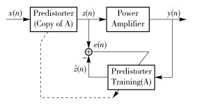
2 Model Identification 2.1 Indirect Learning ArchitectureIndirect learning architecture (ILA) is an efficient method for identifying DPD model. It does not need to construct the PA model, but only uses the output data and input data of PA to estimate the coefficients of a DPD model. Fig. 1[2] shows the block diagram of ILA. In this architecture, DPD model is identified at training block A, and then inserted between original input signal x(n) and PA input. Training block A uses y(n) and z(n) to estimate its coefficients, where y(n) and z(n) are the output and input of PA respectively. (At first, we use x(n) in place of z(n). After the DPD is implemented, we use z(n) to update the coefficients.)
|
Figure 1 Indirect learning architecture of digital predistortion |
From (8) and Fig. 1, "block A" can be expressed as
| $ \begin{align} & \hat{z}\left( n \right)=\sum\limits_{{{q}_{z}}=1}^{{{Q}_{z}}-1}{\sum\limits_{\begin{smallmatrix} {{k}_{z}}=1 \\ {{k}_{z}}=\rm{odd} \end{smallmatrix}}^{{{K}_{z}}}{{{a}_{{{q}_{z}}{{k}_{z}}}}\tilde{z}\left( n-{{q}_{z}} \right){{\left| \tilde{z}\left( n-{{q}_{z}} \right) \right|}^{{{k}_{z}}-1}}}}+ \\ & \ \ \ \ \ \ \ \ \ \ \sum\limits_{{{q}_{y}}=0}^{{{Q}_{y}}-1}{\sum\limits_{\begin{smallmatrix} {{k}_{y}}=1 \\ {{k}_{y}}=\rm{odd} \end{smallmatrix}}^{{{K}_{y}}}{{{c}_{{{q}_{y}}{{k}_{y}}}}y\left( n-{{q}_{y}} \right){{\left| y\left( n-{{q}_{y}} \right) \right|}^{{{k}_{y}}-1}}}} \\ \end{align} $ | (9) |
where
For linearly represented polynomial, it is feasible to extract the coefficients by using linear system estimation theory such as least squares (LS). Sometimes, because of high correlation between each element of the polynomial, the calculation of the inverse matrix tends to be time consuming and unstable. Orthogonal polynomials show great advantages in avoiding numerical instability[12].
LS can be applied to equation-error method directly. For output-error method, we need to set a group of initial coefficients first, and calculate output
Recursive LS (RLS) is a popular adaptive algorithm. Adaptive algorithm is an algorithm which starts from an initial point, and adjusts the coefficients dynamically according to newly sampled input and output. Compared with LS algorithms, adaptive algorithm requires less storage space. Once initial value is properly set, the coefficients always converge to stable states. RLS is also applicable for both equation-error method and output-error method. As a result, we choose RLS to extract the coefficients of (9).
Rewriting (9) in a matrix form:
| $ \mathit{\boldsymbol{\hat z}}\left( n \right) = {\mathit{\boldsymbol{a}}^{\rm{T}}}\mathit{\boldsymbol{u}}\left( n \right) $ | (10) |
where a are the coefficients and u(n) are polynomials of inputs and outputs.
Omitting the tedious and complicated mathematical derivation, the final RLS procedure is
| $ \mathit{\boldsymbol{a}}\left( n \right) = \mathit{\boldsymbol{a}}\left( {n - 1} \right) + \mathit{\boldsymbol{g}}\left( n \right)[z\left( n \right)-{\mathit{\boldsymbol{u}}^{\rm{T}}}\left( n \right)\mathit{\boldsymbol{a}}\left( {n-1} \right)] $ | (11) |
| $ \mathit{\boldsymbol{g}}\left( n \right) = \frac{{\mathit{\boldsymbol{C}}\left( {n - 1} \right){\mathit{\boldsymbol{u}}^ * }\left( n \right)}}{{1 + {\mathit{\boldsymbol{u}}^{\rm{T}}}\left( n \right)\mathit{\boldsymbol{C}}\left( {n - 1} \right){\mathit{\boldsymbol{u}}^ * }\left( n \right)}} $ | (12) |
| $\mathit{\boldsymbol{C}}\left( n \right) = \mathit{\boldsymbol{C}}\left( {n - 1} \right) - \mathit{\boldsymbol{g}}\left( n \right){\mathit{\boldsymbol{u}}^{\rm{T}}}\left( n \right)\mathit{\boldsymbol{C}}\left( {n - 1} \right) $ | (13) |
Equation (13) uses a recursive way to update a(n) which requires less storage memory and improves numerical instability.
Note that in the simulation, equation-error method has a slightly better performance than output-error method, and it is easier to implement. Therefore, allthe following results are calculated by equation-error method.
3 Simulation ResultsIn this section, simulations are implemented to demonstrate the effectiveness of the proposed modified bilinear model. All results presented are simulated in Matlab. Fig. 2 shows the simulation diagram. The input signal is a three-carrier wideband code division multiple access (WCDMA) signal, and it has peak-to-average power ratio (PAPR) of about 6 dB. We will linearize different PA models, including an odd-order-only memory polynomial model and a three-branch parallel Wiener model. The input power is properly adjusted to make the PA to operate at about 5 dB power back off point. During simulation, we first sample the input and output signals of PA. With these signals, we then estimate the proposed DPD model coefficients. Finally, we cascade the proposed DPD model to the PA, and test its performance, including power spectral density, AM/AM characteristic, AM/PM characteristic, normalized mean squared error (NMSE) etc. Additionally, we will compare the proposed DPD model with some widely used DPD models, e.g. MP, GMP.

|
Figure 2 Block diagram of simulation |
Odd-order-only memory polynomial model is expressed as[8]
| $ y\left( n \right)=\sum\limits_{\begin{smallmatrix} m=1 \\ m=\rm{odd} \end{smallmatrix}}^{M}{\sum\limits_{l=0}^{L-1}{{{c}_{ml}}z\left( n-l \right){{\left| z\left( n-l \right) \right|}^{m-1}}}} $ | (14) |
The coefficients are extracted from an actual class AB PA which can be referred from [8].
Set the coefficients [Qz Qy Kz Ky] of (9) to [3 1 3 5]. Fig. 3 shows the power spectral density at the output of the PA with and without a DPD.

|
Figure 3 Power spectral density with and without DPD |
Fig. 3 indicates DPD can bring down the spectral regrowth remarkably.The proposed modified bilinear polynomial model outperforms traditional DPD models obviously.
Tab. 1 lists the number of coefficients and NMSE performance of different DPDs shown in Fig. 3.
|
|
Tab. 1 Comparison for coefficients and NMSE of different DPD models (odd-order-only memory polynomial PA model) |
It can be seen from Tab. 1, GMP uses a large number of coefficients but only gets a small progress compared with MP. However, the proposed modified bilinear model shows great improvement on linearizing PA, and uses the fewest number of coefficients to bring down the NMSE to -65.08 dB.
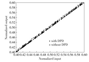
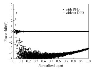
The AM/AM and AM/PM characteristics of PA before and after the proposed DPD are given in Fig. 4 and Fig. 5. It shows that the phase distortion can be decreased very well. (To show AM/AM characteristics clearly, we only draw a part range of the AM/AM plot.)
|
Figure 4 AM/AM characteristics for odd-order-only memory polynomial with and without bilinear model based DPD |
|
Figure 5 AM/PM characteristics for odd-order-only memory polynomial with and without bilinear model based DPD |
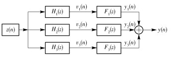
We also use three-branch parallel Wiener model as our PA for comparison. As shown in Fig. 6, Hi (·) is an Linear Time Invariant (LTI) block, and Fi (·) is a memoryless nonlinear block.
|
Figure 6 Parallel Wiener model diagra |
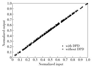
All parameters of this Parallel Wiener model can be referred from [8]. We still set the coefficients [Qz Qy Kz Ky] of (9) to [3 1 3 5]. The rectified AM/AM and AM/PM are shown in Fig. 7 and Fig. 8.
|
Figure 7 AM/AM characteristics for three-branch parallel Wiener model with and without bilinear model based DPD |

|
Figure 8 AM/PM characteristics for three-branch parallel Wiener model with and without bilinear model based DPD |
Furthermore, the number of coefficients and NMSE performance are listed in Tab. 2.
|
|
Tab. 2 Comparison for coefficients and NMSE of different DPD models (three-branch parallel Wiener PA model) |
For three-branch parallel Wiener model, bilinear model still shows the best modeling accuracy. In Tab. 2, bilinear model uses the fewest coefficients and achieves the best NMSE performance.
We use different PAs to test our DPD model. Results show that our modified bilinear polynomial model is efficient and robust for both odd-order-only memory polynomial PA model and a three-branch parallel Wiener PA model. It can compensate the magnitude and phase nonlinearity of PA very well. The most important thing is that it uses relatively fewer coefficients to express high order nonlinearity and deep memory effect than traditional DPD models.
4 ConclusionsA novel model for PA linearization is proposed. This model uses feedback terms to improve its performance. Proper modification is made to the model to decrease its coefficients and fit applications in DPD. Appropriate RLS algorithms are derived to extract coefficients. Simulation results show that the model can effectively linearize PA in both magnitude and phase.
| [1] |
Luo J, Liszewski J, Schubert B. Smart RF signal processing for advanced transmitters: from theory to practice[C]//2012 International Symposium on Signals, Systems, and Electronics. Potsdam: IEEE, 2012: 1-6.
|
| [2] |
Ding L, Zhou G T, Morgan D R, et al. A robust digital baseband predistorter constructed using memory polynomials[J]. IEEE Transation Communications, 2004, 52(1): 159-165. doi: 10.1109/TCOMM.2003.822188 |
| [3] |
Qiao Jianyong. Julia sets and complex singularities of free energies[J]. Memoirs of American Mathematical Society, 2015(234): 1-89. |
| [4] |
Qiao Jianyong. On the preimages of parabolic points[J]. Nonlinearity, 2000(13): 813-818. |
| [5] |
Ai Bo, Zhong Zhangdui, Zhu Gang, et al. A novel scheme for power amplifier predistortion based on indirect learning architecture[J]. Wireless Personal Communications, 2008, 46(4): 523-530. doi: 10.1007/s11277-008-9451-z |
| [6] |
Morgan D R, Ma Z, Kim J, et al. A generalized memory polynomial model for digital predistortion of RF power amplifiers[J]. IEEE Transactions on Signal Processing, 2006, 54(10): 3852-3860. doi: 10.1109/TSP.2006.879264 |
| [7] |
Ai Bo, Zhong Zhangdui, Zhu Gang, et al. Two-dimensional indexing polynomial-based pre-distorter for power amplifiers with memory effects[J]. IET Communications, 2008, 2(10): 1263-1271. doi: 10.1049/iet-com:20080209 |
| [8] |
Ding Lei, Zhou G T, Morgan D R, et al. A robust digital baseband predistorter constructed using memory polynomials[J]. IEEE Transactions on Communications, 2004, 52(1): 159-165. doi: 10.1109/TCOMM.2003.822188 |
| [9] |
Diniz P S R. Adaptive Filtering Algorithms and Practical Implementation[M]. 3rd ed. Boston: Springer, 2008.
|
| [10] |
Lee J, Mathews V J. A stability result for RLS adaptive bilinear filters[J]. IEEE Signal Processing Letters, 1994, 1(12): 191-193. doi: 10.1109/97.338749 |
| [11] |
Ogunfunmi T. Adaptive nonlinear system identification[M]. Boston: Springer, 2007, 118-123.
|
| [12] |
Zhao Xia, He Yabo. Modified gram-schmidt orthogonalization and QR decompositon extraction for digital predistorter[C]//2011 Chinese Control and Decision Conference (CCDC 2011). Mianyang: IEEE, 2011: 1120-1125.
|


