2. Shanghai Niumag Corporation, Shanghai 200333, China;
3. School of Optical Electric and Computer Engineering, University of Shanghai for Science and Technology, Shanghai 200093, China;
4. School of Medical Imaging, Shanghai University of Medicine and Health Science, Shanghai 200318, China
2. 上海纽迈电子科技有限公司, 上海 200333;
3. 上海理工大学 光电与计算机工程学院, 上海 200093;
4. 上海健康医学院 医学影像学院, 上海 200318
As an increasingly important detection method in scientific research and medical diagnostics[1, 2], magnetic resonance imaging (MRI) is more and more popular with practitioners and learners. However, MRI is a complex process involving quantum physics, electronic information science, mathematics, statistics, imaging, etc., which requires learners have enough practical experience as well as theoretical knowledge. Most of MRI teaching and practice relies on the expensive instrument, specific hardware, and enormous time investment. Therefore, to develop a MRI teaching system which is independent on real instrument, while retains operability, is an extremely important pursuit for MRI teaching, learning, and improvement[3, 4].
There have been a few MRI simulation researches reported. Hanson et al.[5] developed a freely available graphical simulator based on the Bloch equations to aid teaching topics ranging from nuclear precession and relaxation to advanced concepts, such as stimulated echoes, spin tagging, and k-space filling. With a graphical interface, users can manipulate spin isochromatic in three-dimensional view by adjusting radiofrequency (RF) pulses and gradients. With the development of computer simulation of multi-channel, multi-dimensional nuclear magnetic resonance (NMR) experiments on a user-defined spin systems, Nicholas et al.[6] employed the Virtual NMR Spectrometer program. The program can carry out most features of modern NMR experiment, such as homo and hetero-nuclear pulse sequences, phase cycling, pulsed field gradients, and shaped pulses. The applications of the Virtual NMR Spectrometer have been illustrated using homo-nuclear COSY, DQF COSY, hetero-nuclear HSQC, and TROSY experiments. Fortin et al.[7] presented an efficient MR angiography simulator for physiological fluids with arbitrarily complex flows. Yoder et al.[8] developed a system that generates images of realistic objects for arbitrary pulse sequences in the presence of factors affecting magnetic field homogeneity, such as magnetic susceptibility, variations in the applied field, and chemical shift, but not including proton density, T1 and T2, etc. Kwan et al.[9] presented a MRI simulator for evaluating image processing and classification, but not for simulating the imaging process of a real instrument. Cao et al.[10] developed a simulator that considers realistic electromagnetic fields when calculating signal, noise, and specific absorption rate based on the Bloch-based MRI system. Liu et al.[11] developed a MRiLab simulator to simulate the design of gradients, RF coil, and RF pulse. But it focused on the parallel operation of three-dimensional imaging, and required a graphic processing unit (GPU) to run the software, which increased the cost and reduced the practicability. Benoit-Cattin et al.[12] developed the SIMRI simulator based on the Bloch equation. It is emphasis on the cause analysis for image artifacts, but not useful for MRI training, because its simulation requires a huge amount of computational power provided by parallel computers. A virtual clinical-like MRI simulation was reported by Hacklander et al.[13] based on three basic physical properties: T1, T2, and the proton density (Pd). It also can simulate convolution artifacts and motion artifacts by changing the sequences and parameters. However, system correction, data acquisition, and original raw data filing were not implemented.
This paper presents a virtual MRI data acquisition and image reconstruction simulation package, naming MRISim. Compared with the other softwares, it conducts similar imaging process like a real MRI instrument, including system correction, data acquisition, raw data filling and image reconstruction, but avoids high expense for instrument and time consuming. Our researches show MRISim is economic and efficient for MRI teaching and training.
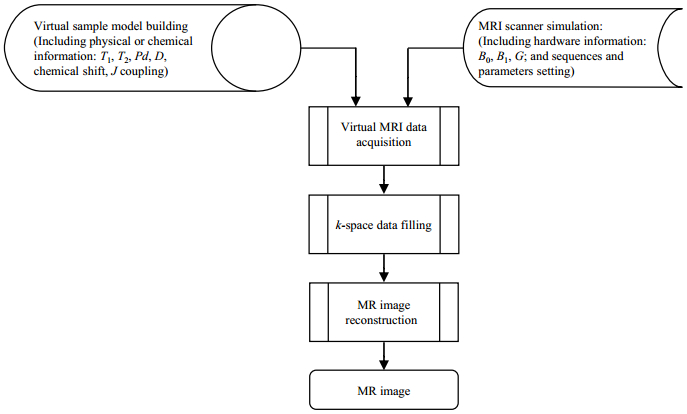
1 Experimental principle and design 1.1 MRISim schematic and functionFig. 1 shows the conceptual framework of MRISim design. It was designed as 5 main parts: virtual sample model building, MRI scanner simulation (induding sequences and parameters setting, and hardware information), virtual MRI data acquisition, k-space data filling, and MR image reconstruction.
|
Fig. 1 Conceptual framework for MRISim design |
The virtual sample model is comprised of a data set with physical and chemical parameters affecting the MR signal, which includes the Pd, T1, T2, self-diffusion coefficient (D), chemical shift and J coupling. In virtual sample model part, the users can select human skull or the other biological or tube samples as sample object, and imaging type (including weighted imaging, fat suppression, black water imaging) to set the basic virtual data parameters.
The MRI scanner simulation considers hardware performance features such as the static magnetic field strength (B0), RF field strength (B1), gradient strength (G), and inhomogeneity of field (delta B0), as well as sequence parameters including the RF pulse length (P1), number of phase encoding (NE), number of sample points (TD), and sweep frequency (SW). The MRI scanner simulation part integrates common pulse sequences used in real MRI scan, such as spin echo (SE), fast spin echo (FSE), gradient echo (GRE), inversion recovery (IR), and echo planner imaging (EPI). Based on the sequence selecting and parameters setting, some imaging technologies having been applied, such as tissue suppression, rally point, half Fourier scanning, and black-water, water image can be performed.
Then, the users can perform virtual data acquisition as using a real MRI scanner.
In k-space data filling part, the users can fill it with line fill, spiral fill, and radial fill strategies.
In MR image reconstruction part, the basic 2D fast Fourier transform (FFT) algorithm was used to reconstruct the image from k-space data. For spiral fill and radial fill strategies, before 2D FFT, the k-space data should be taken girding transformation.
Besides those above, 11 kinds of artifact causes including truncation, aliasing, chemical shifts, RF interference, etc. can be analyzed through direct simulation for the errors.
1.2 Intrinsic composition modelA gray contrast image of soft tissue can be obtained based on the intrinsic characteristics of the biological tissue combined with the pulse sequence. Therefore, an intrinsic composition model should first be established to provide virtual samples for subsequent processing.
We first select high-resolution MR images to ensure the authenticity and reliability of the virtual sample structure, and use threshold segmentation to obtain the structural morphology for different compositions. While the high-resolution data matrix can be handled accurately on the computer, it is so large that the running speed is significantly impacted. Therefore, we adopt a ratio compression algorithm to reduce the array size [5]. Finally, to replace the gray of regions of interest for building the structure composition model, we use tissue values for Pd, T1, and T2.
When MRI training, samples are often placed inside two concentric test tubes, as shown in Fig. 2(a), to provide differential absorption effects. Therefore, the MRISim model also provides this test tube mode, and the users can choose water, oil, muscle, fat, cerebrospinal fluid, etc., as individual materials in the test tubes. In addition, MRISim offers another simple model of rectangular section samples [Fig. 2(b)], and more complex models such as a human skull [Fig. 2(c)] incorporating fat, meninges, gray matter, white matter, cerebrospinal fluids, and bones, or a spine model [Fig. 2(d)] incorporating spinal cord, vertebral body, and intervertebral discs as well.

|
Fig. 2 Structure composition of sample models in MRISim. (a) Water-oil tube sample; (b) Water-oil rectangular section sample; (c) Human skull; (d) Human spine |
An MR image is composed of pixels with position and intrinsic compositional information. Therefore, the spatial orientation must be understood before analyzing the data. Fig. 3(a) shows a selected layer under RF pulse excitation. The phase (ϕ) and frequency (f) for each pixel are the same, and thus the pixel location cannot be distinguished. Then a phase encoding gradient along the y axis [Fig. 3(b)] and a frequency encoding gradient along the x axis [Fig. 3(c)] are applied to provide a unique initial phase and frequency for each pixel[14]. The accumulation for each voxel signal is the same as the usual NMR [15]:
| $ S({t_m},D) = A\sum\limits_{y = 1}^i {\sum\limits_{x = 1}^k \rho \cos [({\omega _0} + \gamma x{G_x}){t_m} + \gamma y{G_y}{D_y}]\exp (\frac{{ - {t_m}}}{{{T_2}}})} $ | (1) |

|
Fig. 3 Spatial orientation. (a) The original layer, the phase and frequency of each pixel are the same; (b) After phase orientation, pixels have different phases along the y axis; (c) After frequency orientation, pixel have different frequencies along the x axis |
where A is the amplification factor; tm is the frequency coding discrete sampling time; Dy is the phase encoding time; i and k are the row and column numbers of the image matrix, respectively; ρ represents the proton density (Pd); Gx and Gy are the strength of frequency encoding gradient and phase encoding gradient, respectively; γ is the gyromagnetic ratio of observed nucleus.
The signal is obtained in the NMR receiving unit through a mixing and low pass filter to eliminate the Larmor frequency:
| $ I({t_m},D) = A\sum\limits_{y = 1}^l {\sum\limits_{x = 1}^k \rho \cos (\gamma x{G_x}{t_m} + \gamma y{G_y}{D_y})\exp (\frac{{ - {t_m}}}{{{T_2}}})} $ | (2) |
By phase detection, the real part is shifted 90° and then the imaginary part signal is obtained:
| $ Q({t_m},D) = {\rm{j}}A\sum\limits_{y = 1}^l {\sum\limits_{x = 1}^k \rho \sin (\gamma x{G_x}{t_m} + \gamma y{G_y}{D_y})\exp (\frac{{ - {t_m}}}{{{T_2}}})} $ | (3) |
Where j is the imaginary unit.
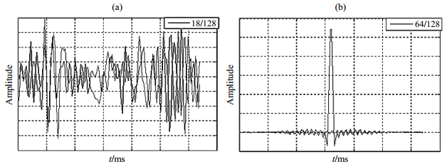
Following the established mathematical model, we can get the original k-space data using MRISim software. For example, supposing the skull model was scanned with phase encoding gradient set to 128 (the number of phase encoding step, other parameters are default), the MRI signal can be dynamically displayed in the interface, as shown in Fig. 4. Fig. 4(a) and 4(b) show the signal of 18th and 64th phase encoding step separately.
|
Fig. 4 MRI data acquisition. (a) The 18th phase encoding step with lower signal to noise ratio; (b) The 64th phase encoding step with higher signal to noise ratio |
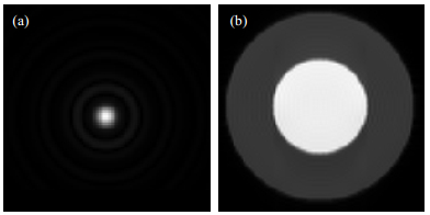
k-space (raw data space) is filled with MRI signal from a layer of sample by a line-fill track[16]. The k-space data of the sample water and oil tube model is shown in Fig. 5(a), each line of which is a two-dimensional function[17]:
| $ S'({t_m},{D_y}) = I({t_m},{D_y}) + Q({t_m},{D_y}) $ | (4) |
|
Fig. 5 k-space data filling for the sample water and oil test tube model. (a) Raw grayscale MR image; (b) Fourier transformed image |
Converted Equ. (4) into a matrix expression as follows:
| $ S({t_m},{D_y}) = A\sum\limits_{y = 1}^i {\sum\limits_{x = 1}^k \rho \exp [{\rm{j}}(\gamma x{G_x}{t_m} + \gamma y{G_y}{D_y})]\exp (\frac{{ - {t_m}}}{{{T_2}}})} $ | (5) |
If setting
| $ S({t_m},D) = A\sum\limits_{{\omega _x}} {\sum\limits_{{\omega _y}} \rho } \exp [{\rm{j}}({\omega _x}{t_m} + {\omega _y}{D_y})]\exp (\frac{{ - {t_m}}}{{{T_2}}}) $ | (6) |
The location (ωx, ωy) for an individual pixel can be demodulated by the Fourier transform of S and ρ, as shown in Fig. 5(b).
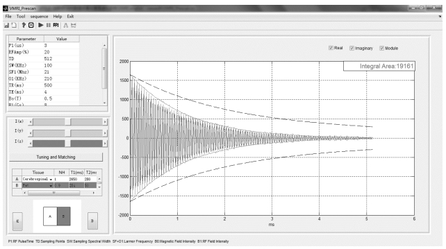
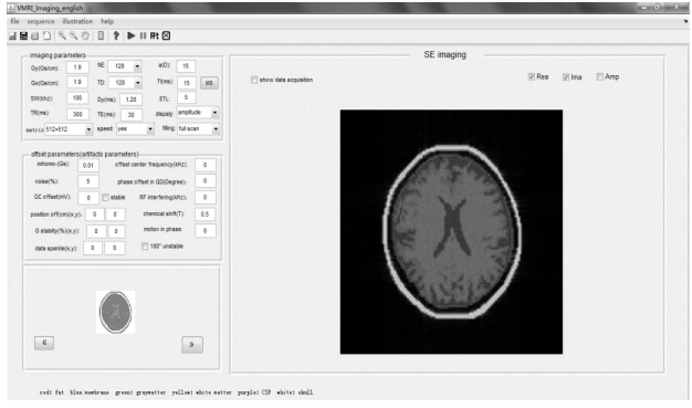
1.5 Interface modules of MRIsimThe user interface modules of MRISim software are composed of theory demonstration, pre-scan (Fig. 6), probe tuning and matching, and imaging (Fig. 7) interfaces.
|
Fig. 6 Pre-scan interface module of MRISim |
|
Fig. 7 Imaging interface module of MRISim |
In the pre-scan interface, users can select the sample model, compositional characteristic values, and parameters to obtain free induction decay (FID), SE, or CPMG signals based on RF pulses.
In the probe tuning and matching interface, users should orderly select different wires to produce a solenoid coil with different diameter, height, and gap, decide upon a series or parallel resonance circuit, tune the capacitor matching, and observe the impedance and reflection coefficients.
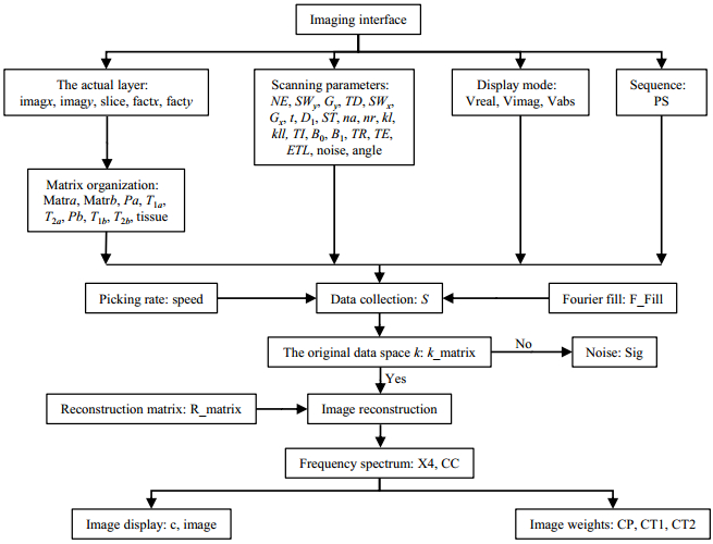
In the imaging interface, users can select the image sequences (SE, FSE, IR, and so on), set the scanning parameters [repetition time (TR), echo time (TE), SW, and so on], and choose the target data. After k-space data filled, upon clicking the 'FFT' button, users will obtain the MR images. Fig. 8 shows the signal processing flowchart.
|
Fig. 8 Image processing flowchart of MRISim |
The software was developed using Matlab2016a, and can run on the 64-bit window system with larger than 4G random access memory (RAM). The readers can acquired the demo version of MRISim by Email to the first author.
2 DiscussionThe original aim of this project was the virtualization of an MRI instrument with the same operational process and performed as a real device. Therefore, the interface and tool buttons on the real instrument were copied to the MRISim interface to provide an ideal experimental based teaching environment. We visualized the processes of system correction, data acquisition, and k-space filling to demonstrate the principles of MRI. In addition, MRISim software can simulate the causes and outcomes for 11 MRI artifacts that are not available in other software systems. Using this simulator, 15 experimental projects can be performed like operating a real bench-top MRI instrument, which can be categorized into three types: system correction projects, imaging projects and artifacts analysis projects.
2.1 System correction projectsSystem correction is the key process for any clinical MRI scan because it is critical for MRI image quality. Based on this software, by using pre-scan module, students can manually carry out the four steps of MRI system correction: NMR signal detection and RF center frequency determination, RF angle adjustment, active shimming, and auto tuning and matching of RF coil.
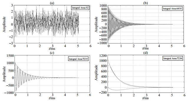
For example, NMR signal detection and RF center frequency determination project, in other word to measure the Larmor frequency, the user can adjust the frequency offset manually and observe the FID shape change. If the Larmor frequency is not within the RF bandwidth range, the resonance condition is not satisfied, so there has no signal just noise like Fig. 9(a). If there is large differential between the Larmor frequency and RF center frequency, the FID oscillation frequency is high due to deviating from the ideal resonance condition as shown Fig. 9(b). On the other hand, if the signal oscillation frequency is low, this implies near resonance like Fig. 9(c), and it is only when the Larmor and RF center frequencies are equal that the signal decays exponentially and the nuclear magnetic resonance phenomenon occurs like Fig. 9(d).
|
Fig. 9 The FID signal shape stimulated by different RF center frequency. (a) Only noise because of Larmor frequency not within the RF bandwidth range; (b) High signal oscillation frequency; (c) Low signal oscillation frequency; (d) RF center frequency is equal to Lamer frequency |
By using imaging interface, students can manually carry out the MRI imaging projects, such as acquiring images with different resolution, different weighting by adjusting related parameters using different sequence.
2.2.1 Image resolution adjustmentPrior to MRI, medical imaging personnel would manually adjust the field of view (FOV) according to the sample size to precisely display the imaged area and achieve good image resolution. During operation, FOV is affected by many imaging parameters, including Gy, Gx, Dy, and sampling spectral width (SWx). Therefore, these parameter settings are included in the MRISim software, which help users to better understand the effects of sampling parameters on an image. Users can select different parameters and immediately observe the image effects.
Fig. 10(a) shows the SE sequence and default parameters (Gx = Gy= 1.9×10⁻⁴ T/cm, Dv = 1.28 ms, SWx = 100 kHz) to scan the human skull, and Fig. 10(b) shows that when Gy increased to 2.3×10⁻⁴ T/cm, with all other parameters staying constant, the vertical FOV was reduced, and the resulting MR image was vertically elongated. Thus, as Gy increases, FOV decreases in vertical direction, but the vertical spatial resolution improves. Fig. 10(c) shows that when SWx was reduced to 50 kHz, the horizontal FOV decreased. Thus, reducing SWx can improve the horizontal spatial resolution. Fig. 10(d) shows that when Gx increased to 5×10⁻⁴ T/cm, part of the image folded, called a wraparound artifact. Thus, although increasing Gx can reduce the horizontal FOV and improve spatial resolution, the wraparound artifact can arise when the FOV is too small and the signal from outside the FOV wraps to another side of the image.

|
Fig. 10 Effects of scanning parameters on MR image shape, for the human skull model: (a) Regular image; (b) Elongated in the phase encoding direction with Gy increased; (c) Elongated in the frequency encoding direction with SWx reduced; (d) Wraparound artifact in the frequency encoding direction with Gx increased |
Therefore, the MRISim software allows users to investigate different parameter settings and to directly observe changes in MR image shape and resolution, which can help users develop a solid knowledge for practical imaging.
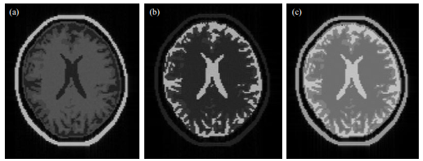
2.2.2 Image weighting adjustmentIn the SE sequence, we can select TR and TE to acquire soft tissue images for a contrast of Pd, T1, or T2, and to selectively observe tissue structures. In theory, short TR and TE will provide T1 weighted images, long TR and TE will provide T2 weighted images, and long TR with short TE will provide Pd weighted images. However, it is difficult for learners to relate theoretical knowledge with actual MR images, and capturing multiple images of the same object is time consuming and practically onerous. Therefore, practical imaging experience and a visualization of effects can greatly improve understanding of SE weighted images.
Fig. 11(a) shows a T1 weighted image of the human skull model (TR=200 ms, TE=10 ms), highlighting white matter in the brain. Fig. 11(b) shows a T2 weighted image (TR=6 000 ms, TE=100 ms), highlighting cerebrospinal fluid. Fig. 11(c) shows a Pd weighted image (TR=6 000 ms, TE=15 ms), which highlights the entire brain appearance except for the skull, i.e., there is not much difference in proton density in brain tissues.
|
Fig. 11 Different image weighting using SE sequence: (a) T1 weighted image; (b) T2 weighted image; (c) Pd weighted image |
Thus, Pd and T2 weighted images require a long TR, which in practice requires very long image acquisition time. However, imaging time of MRISim software is regardless of the different weights. Rapid image generation can greatly increase the efficiency of experimental learning.
2.2.3 Different image sequenceIn image module of MRISim, 8 typical sequence, such as SE, FSE, IR, 1D frequency encoding sequence, IR, GRE, EPI and spiral EPI, can be selected to carry out the projects by manually adjusting related parameters. Here we only take IR sequence as an example.
The main difference in the IR sequence, from the SE sequence, is that a 180˚ pulse is applied before the 90° pulse. The original magnetic vector along the z axis flips to the -z direction due to the 180˚ pulse, and the dynamic range of the vertical magnetization is doubled, ranging from M0 to -M0. The time between the two pulses is the inversion time (TI). Users can produce images of different weights by adjusting the TI.
Although the IR sequence can provide images of different weights by adjusting TI, practical application of this sequence is limited due to long acquisition time. Clinically, the IR sequence is mainly used to suppress the signal from fat and water. The IR sequence is also occasionally used to differentiate the boundary between different structures by bounce point imaging to acquire boundary information from different tissues.
The speed of image acquisition using the IR sequence is very slow in practical hardware imaging experiments, which significantly reduces learning efficiency. However, as with the SE case, MRISim software allows users to practice different imaging techniques using the IR sequence with little or no time penalties, including fat suppression, water suppression, and bounce point imaging. Fig. 12 shows a water and oil sample scanned at TR=8 000 ms, TE=10 ms, and with different TI. Fig. 12(a) (default TI=15 ms) shows that although high contrast between the water and oil was achieved, we cannot see the individual components in the image. Fig. 12(b), with TI=ln2×T1f, where T1f indicates the T1 value of fat, shows that the oil signal was suppressed and appeared the same as the background, i.e., a fat suppressed image. In Fig. 12(c), with TI=ln2×T1w, T1w indicates that the T1 value of the water signal was suppressed, i.e., in a water suppressed image. In Fig. 12(c), TI=550 ms. The oil magnetization vector relaxed across 0, whereas the vector for water did not. The absolute value of the two vectors were the same, with opposite directions, and hence a bounce point image was acquired. Thus, the image shows both components with same signal level, and a clear boundary can be observed [Fig. 12(d)].

|
Fig. 12 Images acquired for the IR sequence from the test tube model: (a) Regular T1 weighted image; (b) Fat suppressed image; (c) Water suppressed image; (d) Black ring appeared at the oil and water boundary |
Using the MRISim software, users can analyze the causes for more than 11 types of MRI artifacts, including truncation, aliasing, center shift, chemical shift, mirror, zipper, RF interference, stripe, motion, etc. By setting the relative offset, hardware, or software parameters for acquisition, different performances of different artifacts are provided. We discuss a simple example of stripe artifacts to illustrate this function. Other artifacts analysis examples can be seen in the Simulation Experiment on Medical Imaging Principle textbook which pressed by Peoples Health Public House in August 2018.
Stripe artifacts arise from a single spark when the circuit discharges during analog to digital converter sampling, and one data point of k-space shows an abnormal high or spike signal. Stripe artifacts are displayed as light fringes and shade overlays on the sample image. Depending on the spike location in k-space, the stripe shows a different direction (longitude, transfers, or oblique), and a different gap. For example, Fig. 13 shows the stripe artifacts from separate spike locations set at (60, 60), (36, 96), (24, 108), and (118, 118) [Fig. 13(a)~(d), respectively]. The different positions result in stripes with a different direction and gap.

|
Fig. 13 Stripe artifacts arising from different spike locations. (a) (60, 60); (b) (36, 96); (c) (24, 108); (d) (118, 118) |
A bench-top MRI instrument was developed by Li Gengying (first author's doctoral tutor) team for teaching in 2002[18]. During 7 years of experiments and teaching experience, some problems and weakness of the instrument were discovered, and the idea of virtualization of a mini-type MRI scanner emerged. After 3 years, the development of MRISim was completed.
3 ConclusionFor educational and training purposes, this simulator system dynamically displays the data acquisition and k-space data filling processes as a real equipment, and avoids hardware weaknesses while providing similar imaging results like using a real instrument. Furthermore, it can be operated more readily than a real instrument.
The software package avoids many of the problems associated with hardware imaging experiments, such as magnetic field inhomogeneity, long acquisition time, and limitations in the number of imaging devices. Without requiring a hardware device, the software can generate similar results to that from the real device. This provides MRI practitioners and trainees with a platform for quick and efficient training and practicing. In addition, as the software improves and matures, it will be able to further provide clinicians with pre-calibrated standard parameters and imaging sequences for particularly desirable tissue contrasts. MRI physicians can also use this software to assist in clinical diagnosis. The virtual image interface helps users to develop a deeper understanding of the MRI process by allowing them to observe the effects of different signals, k-spaces, image sequences, tissues, and other parameters, thereby teaching them how to more effectively apply MRI technology.
So MRISim can be thought as an effective tool for conducting MRI experiments on a computer, thereby avoiding high expense of hardware and time-consuming on real MRI instruments. MRISim is also an efficient and reliable tool that can be used for training MRI operators, engineers, and graduate students.
Furthermore, the sample model of this project is to assign values to different tissue's biophysical information (Pd, T1, T2, D). There are some differences between these value and the real value of body tissue, but this is enough for training and teaching. In future, we will get more authentic data of a real body through mapping technologies of a clinical MRI scanner, then the results derived from the simulator can be used in medical imaging diagnostic services.
| [1] | ZU D L, GAO J H. Nuclear magnetic resonance (NMR) imaging physics principle and method[M]. Beijing: Peking University Press, 2014. |
| [2] | STOCKER T, VAHEDIPOUR K, PFLUGFELDER D, et al. A high performance computing MRI simulations[J]. Magn Reson Med, 2010, 64(1): 186-193. DOI: 10.1002/mrm.22406. |
| [3] |
KUANG B, HE C M. A perception on the development of the virtual scan technology for the magnetic resonance imaging[J].
Chinese J Magn Reson Imaging, 2011, 2(3): 218-224.
匡斌, 何超明. 磁共振成像虚拟扫描技术的发展及趋势浅淡[J]. 磁共振成像, 2011, 2(3): 218-224. DOI: 10.3969/j.issn.1674-8034.2011.03.012. |
| [4] | SHUI L. The design and realization of platform of magnetic resonance imaging[J]. Software Guide, 2014, 13(6): 147-150. |
| [5] | HANSON L. A graphical simulator for teaching basic and advanced MR imaging techniques[J]. Radiographics, 2007, 27(6): e27. DOI: 10.1148/radiographics.27.6.e27. |
| [6] | NICHOLAS P, FUSHMAN D, RUCHINSKY V, et al. The virtual NMR spectrometer:a computer program for efficient simulation of NMR experiments involving pulsed field gradients[J]. J Magn Reson, 2000, 145(2): 262-275. DOI: 10.1006/jmre.2000.2108. |
| [7] | FORTIN A, SALMON A, BARUTHIO J, et al. High performance MRI simulation of arbitrarily complex flow:A versatile framework[J]. HAL, 2016. |
| [8] | YODERD, ZHAO Y, PASCHAL C, et al. MRI simulator with object-specific field map calculations[J]. Magn Reson Imaging, 2004, 22(3): 315-328. DOI: 10.1016/j.mri.2003.10.001. |
| [9] | KWAN R K, EVANS A C, PIKE G B. MRI simulation-based evaluation of image-processing and classification methods[J]. IEEE T Med Imaging, 1999, 18(11): 1085-1097. DOI: 10.1109/42.816072. |
| [10] | CAO Z, OH S, SICA C, et al. Bloch-based MRI system simulator considering realistic electromagnetic fields for calculation of signal, noise, and specific absorption rate[J]. Magn Reson Med, 2014, 72(1): 237-247. DOI: 10.1002/mrm.24907. |
| [11] | LIU F, KIJOWSKI R, BLOCK W. Performance of multiple types of numerical MR simulation using MRiLab[C]. ISMRM, 2014: 5244. |
| [12] | BENOIT-CATTIN H, COLLEWET G, BELAROUSSI B. The SIMRI project:a versatile and interactive MRI simulator[J]. J Magn Reson, 2005, 173(1): 97-115. DOI: 10.1016/j.jmr.2004.09.027. |
| [13] | HACKLANDER T, METENS H. Virtual MRI:a PC-based simulation of a clinical MR scanner[J]. Acad Radiol, 2005, 12(1): 85-96. DOI: 10.1016/j.acra.2004.09.011. |
| [14] | 陈武凡, 康立丽. MRI原理与技术[M]. 北京: 科学出版社, 2012. |
| [15] | 张学龙. 医学影像物理学教程[M]. 北京: 科学出版社, 2013. |
| [16] |
WANG J, WANG X. The MATLAB-based rapid method of three-dimensional reconstruction of MRI images[J].
Journal of Taishan Medical College, 2012, 3(7): 515-517.
王军, 王昕. 一种基于MATLAB的快速MRI图像三准重建方法[J]. 泰山医学院学报, 2012, 3(7): 515-517. DOI: 10.3969/j.issn.1004-7115.2012.07.010. |
| [17] | MATT A, BERNSTEIN B, KEVIN F, et al. Handbook of MRI pulse sequences[M]. USA: Elsevier Academic Press, 2004. |
| [18] |
XIAO P F, SHEN J, JIANG Y, et al. Bench-top magnetic resonance imaging system[J].
Chinese J Magn Reson, 2002, 19(4): 345-352.
肖鹏飞, 沈杰, 蒋赟, 等. 台式磁共振成像系统的研制[J]. 波谱学杂志, 2002, 19(4): 345-352. |
 2019, Vol. 36
