Air pollution caused by urbanization and industrialization has exerted significant impacts on public health and well-being, which has been widely acknowledged by both the governmental authorities and the scientific communities.To understand the atmospheric pollution level and evaluate the air quality, it is of great importance to provide scientific information about the air pollutant concentration, especially in the densely populated urban areas. During the past two decades, the Chinese environmental authorities made a lot of efforts to strengthen environmental management and issued a series of environmental policies, one of which was the transformation from the air pollution index (API), the national ambient air quality standard released in 1996, to the new standard of air quality index (AQI) in 2012 (MEP, GB 3095-2012).
The newly applied AQI in China, which monitors six pollutants in ambient air, namely PM2.5, carbon monoxide, sulphur dioxide, nitrogen dioxide, PM10, and ozone, has been widely used in countries worldwide[1-2]. However, some researchers remarked its limitations in illustrating the air pollution level[3-4]. They argued that the AQI was computed by the value of the pollutant with the highest concentration relative to its standard on a given day, which failed to report the whole situation of populations exposed to all pollutants, and they suggested that the comprehensive and aggregate indices taking all the pollutant concentrations into consideration should be deeply discussed[5-8]. Some researchers proposed new indicators in light of the potential impacts of poor air quality on human health, and others explored new methodologies to measure the characteristics of all air pollutants[9-12]. Nevertheless, how to quantify air quality scientifically and comprehensively is still an open field that needs deep concern.
Empirical studies have illustrated the spatial patterns and temporal characteristics of the urban air quality in China in terms of one pollutant concentration or comprehensive indices in accordance to the new standards of GB 3095-2012, but comparison research between different indices has not been well addressed so far[13-15]. Another important domain in the literature is to explain the driving factors behind urban air quality and regional differentiation, which can be divided into two important perspectives, namely natural perspective and socio-economic perspective[16]. From the meteorological perspective, natural factors such as annual precipitation, annual average relative humidity, atmospheric circulation, etc., have been reported to significantly impact the urban air quality[17-20]. Some authors argued that, given the same natural condition, socio-economic factors, such as urbanization level and industrialization, played more important roles in air quality improvement[21-26]. Other authors pointed out that the environmental regulation and the market-oriented economy were mutually constrained, which shaped the pattern of urban air pollution in China[27-29]. Since socio-economic factors connect air quality control with urban planning and environmental regulation, it is necessary and practical to illustrate the impacts of socio-economic variables on air quality, which still requires in-depth investigations.
In this study, we attempt to evaluate the urban air quality in China, illustrate their spatial characteristics in terms of two systems of air quality indices, namely AAQI (aggregate air quality index) and AQI (air quality index), and further to examine the main determinants driving variations of air quality. In section 1, firstly, we provide a comparison evaluation of the urban air quality for 113 key environmental protection cities in China in respects of the two versions of air quality indices. Furthermore, the panel data regression models are constructed to test the determinants driving regional variations of air quality in China. The findings in our study are expected to identify the superiority of different air quality measurements and to have significant implication for regional air quality evaluation and environmental management.
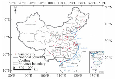
1 Materials and methods 1.1 Data sourceIn this research, datasets of 113 key environ-mental protection cities in China mainland were collected. Classified by China central government from the 11th Five-Year Plan, the key environmental protection cities have targeted at promoting air quality and have adopted a series of pollution prevention policies. These 113 sample cities include the capital (Beijing), municipalities (Shanghai, Tianjin, and Chongqing), 27 province capitals and other 82 economically important cities (Fig. 1). Accordingly, their air quality can generally outline the situation of urban air quality in China and that is why they were chosen as sample cities in this paper. The monitoring data of annual air quality and the explanatory variables of air quality in regression models were collected from China Statistics Yearbook, China Statistics Yearbook on Environment and Chinese City Statistical Yearbook. Spatial variation and its driving factors analyzed in this paper were conducted in ArcGIS 10 and Stata 14, respectively.
|
Download:
|
|
Fig. 1 Spatial distribution of 113 sample cities |
|
To report the air pollution situation to public, researchers have put forward different forms of air quality indices in calculation, which can be divided into two categories as single pollutant index and multi-pollutant index.
IAQI (individual air quality index), an air quality index of individual pollutant, is calculated as
| $ \mathrm{IAQI}=\frac{\left(\mathrm{IAQI}_{\mathrm{H}}-\mathrm{IAQI}_{\mathrm{L}}\right)}{\left(C_{p \mathrm{H}}-C_{p \mathrm{L}}\right)} \times\left(C_{p}-C_{p \mathrm{L}}\right)+\mathrm{IAQI}_{\mathrm{L}}, $ | (1) |
where, Cp is the rounded concentration of pollutant p; CpH is the breakpoint that is greater than or equal to Cp; CpL is the breakpoint that is less than or equal to Cp; IAQIH refers to the air quality index value corresponding to CpH; and IAQIL refers to the air quality index value corresponding to CpL (the threshold values of IAQIH, IAQIL, CpH and CpL are shown in Table 1).
|
|
Table 1 The upper limits of AQI values and corresponding pollutant concentrations |
Air quality index (AQI), which is commonly used worldwide to communicate how polluted the air currently is, is calculated by reference to various pollutants and its value depends on the maximum of the IAQI of all pollutants, which is shown as
| $ \mathrm{AQI}=\max \left(\mathrm{IAQI}_{1}, \mathrm{IAQI}_{2}, \cdots \mathrm{IAQI}_{x} \cdots \mathrm{IAQI}_{n}\right) $ | (2) |
where, IAQIx refers to air quality index of individual pollutant x, corresponding to SO2, NO2, PM10, CO, O3 and PM2.5, respectively; and n is the number of pollutants.
Since AQI is reported for the ambient pollutant index depending on themaximum pollutant, it could not depict the comprehensive air quality regarding all monitored pollutants. In order to compare urban air quality differentiation in China, we computed another air quality index named as AAQI (aggregate air quality index) for each sample city. Proposed by Swamee and Tyagi[11] and further developed by Kyrkilis[9], AAQI takes the combined effects of all criteria pollutants into account, which is shown as
| $ \mathrm{AAQI}=\left(\sum\limits_{i=1}^{n}\left(\mathrm{IAQI}_{i}\right)^{\rho}\right)^{\frac{1}{\rho}}, $ | (3) |
where, IAQIi is the index of i-th pollutant; ρ is a pollutant irrelevant constant.
In an extreme case of ρ=1, the AAQI becomes a linear summation of all IAQI. And if ρ=∞, the AAQI would equal to the maximum IAQI of all criteria pollutants, which is same as the AQI defined in the Eq. (2). How to determine the appropriate value of ρ is important and it is still an open scientific topic. In most of the existing studies, it is commonly suggested that the value of ρ should be between 2 and 3. Accordingly, we set the value of ρ=2.5 in this study.
1.2.2 Spatial interpolationSpatial interpolation, a data estimation method widely used in geo-statistics, is based upon the theory that values in near-by locations are more similar or related than values that are far apart. On the basis of this theory, spatial interpolation procedure estimates the values of unknown points in an area by computing the data of nearer known points that influence the unknown points[30]. To illustrate the spatial variation of urban air quality in China, we use Kriging procedure, whose advantage is that it can generate an estimated surface from a scattered set of points[31], and hence the general regional differentiation of urban air quality in China can be depicted. The limitation of Kriging interpolation is that there might be significant errors when the estimated region has less sample points. But to generate the overall spatial pattern, Kriging is still an efficient estimation method for the spatially local interpolation, by which regional differentiation of urban air quality in China can be described.
1.2.3 Regression modelsTo further understand the variations of urban air quality in China, panel data models were used to detect the various influential factors. To select explanatory variables having significant impacts on air quality, typical socio-economic factors described from theoretical perspective and previous literature were tested by canonical correlation analysis and Pearson correlation. According to the results, 8 significant variables were identified from possible explanatory variables based on the significant test of correlation coefficients and they were classified into four categories, which are urbanization level, industrial structure, environmental regulation and natural condition (Table 2). To further investigate the significance of these explanatory variables, three panel data models, which could capture the complexity of different factors by comparing with cross-sectional or time-series data, were used to process the data related to the sample cities.
|
|
Table 2 Explanatory variables for regional variation of urban air quality and their Pearson correlation coefficients |
Model 1: pooled regression model
Pooled regression model uses OLS regression which is accustomed to the cross-sectional data to process the panel data. Since pooled regression model assumes no individual effect, the explanatory variables for different samples and sections are irrelative to the individual heterogeneity. The pooled regression model is expressed as
| $ Y_{i t}=\alpha+\sum\limits_{m=1}^{k} \beta_{m} X_{m i t}+\theta_{i t}, $ | (4) |
where, m=1, 2, …, k is the explanatory variable, Xmit is the explanatory variable m of individual i in time t, Yit is explained variable of individual i in time t, and θit is the varying random error term depending on individual i and time t.
In the pooled regression model, α is irrelevant to all the explanatory variables Xmit.
Model 2: fixed effect model
When the panel data model takes the individual-specific effects into consideration, the intercept terms are varied depending on the different samples but the slope coefficients being same, and the panel data model is called individual fixed effect model, shown as
| $ Y_{i t}=\alpha_{i}+\sum\limits_{m=1}^{k} \beta_{m} X_{m i t}+\theta_{i t}, $ | (5) |
where, m, k, Xmit, Yit and θit are the same as in Eq. (4).
In the individual fixed effect model, αi is the parameter which would be changed with the changing individual i.
Individual fixed effect model solves the missing variables which are time invariant but individual varying. Analogously, time fixed effect model could solve the missing variables which are individual invariant but time varying. When the panel data model takes both individual fixed effect and time fixed effect into consideration, it is called two-way fixed effects model, shown as
| $ Y_{i t}=\alpha_{i}+\gamma_{t}+\sum\limits_{m=1}^{k} \beta_{m} X_{m i t}+\theta_{i t}, $ | (6) |
where, m, k, Xmit, Yit and θit are the same as in Eq. (4), αi is the same as in Eq. (5).
In the two-way fixed effects model, γt is the dummy variable defined by time t.
Model 3: random effect model
In the random effect model, the hypothesis is that the effect of stochastic factors would not be varied with time change, and it is irrelevant with the random error terms. The random effect model is shown as
| $ Y_{i t}=\alpha_{i}+\sum\limits_{m=1}^{k} \beta_{m} X_{m i t}+\theta_{i t}, $ | (7) |
where, m, k, Xmit, Yit and θit are the same as in Eq. (4).
In the random effect model, αi is regarded as the intercept term containing individual heterogeneity which is irrelevant to all the explanatory variables Xmit.
2 Results and analysis 2.1 Annual variation of air quality in light of different indexTable 3 lists the descriptive statistics of urban air quality in terms of AQI and AAQI. It shows a general downward trend in both the annual mean and the standard deviations, which indicates a desirable evolution of urban air quality in general and a gradually narrowing differences of air quality among different cities.
|
|
Table 3 Descriptive statistics of AQI and AAQI of sample cities in China |
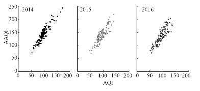
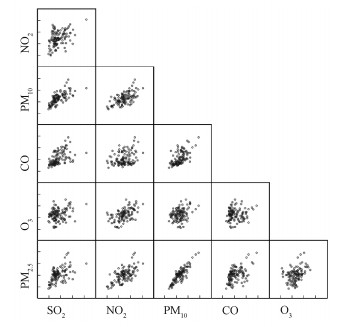
As shown in Fig. 2, AAQI was closely related to AQI, whose rank correlation coefficients are 0.905 in 2014, 0.874 in 2015 and 0.886 in 2016, respectively. Even though the AQI is calculated in terms of the maximum pollutant concentration, the close correlations between different pollutants lead to the high positive relationship between AQI and AAQI, as shown in Fig. 3. Accordingly, AAQI is as effective as AQI when it comes to describe the urban air quality in general perspective.
|
Download:
|
|
Fig. 2 Scatter diagram of AQI and AAQI in China (2014-2016) |
|
|
Download:
|
|
Fig. 3 Scatter diagram of concentrations of the six air pollutants in sample cities (in 2016) |
|
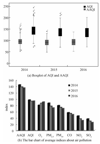
Moreover, when it comes to the cities with extreme air quality indices, there is slight difference that the outliers of AAQI almost matched those of AQI, as shown in Fig. 4(a) and Table 4. Abnormal values occurred on cities as Shijiazhuang, Handan, Baoding and Haikou synchronously in 2014, and concurred on Baoding city in 2015. Besides, the outliers of AAQI show an obvious stratification according to numerical value analysis.
|
Download:
|
|
Fig. 4 Comparison among different air quality indices (2014-2016) |
|
|
|
Table 4 Outliers of AQI and AAQI |
Figure 4(b) illustrates a downward trend of IAQI except O3. The average indices of SO2, NO2, CO, PM10 and PM2.5 have been decreasing from 2014 to 2016. The average indices of SO2 and NO2 have dropped by more than 31%, while the average index of PM2.5 has fallen by 17.6%. Furthermore, the average indices of PM10 and CO have decreased by more than 10%. On the contrary, the average index of O3 has increased by 12.6%, which tends to be closely related to the growth of urbanization level and the mixed effect of urban air pollutants. In general, the variation of AAQI matched that of individual air pollutants. By contrast, the average of AQI was the lowest in 2015, which did not match that of individual air pollutants. Since AQI does not depict all the monitored pollutants, this deviation is acceptable.
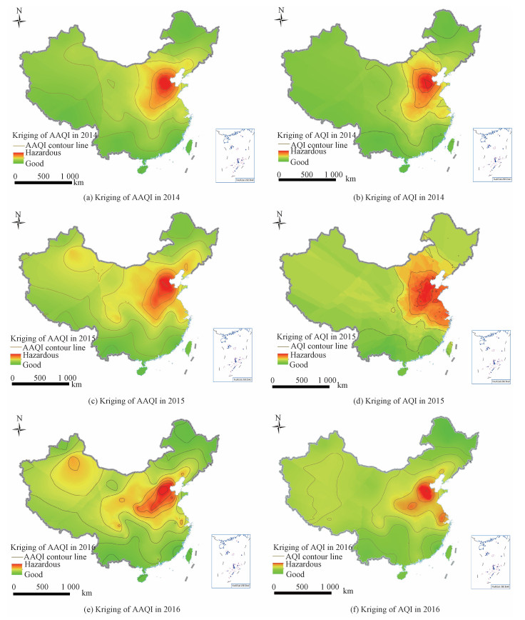
2.2 Spatial characteristics of urban air qualityIn our study, Kriging and contour map were utilized to analyze the spatial evolution of urban air quality. Figure 5 illustrates the geographical feature of urban air quality, showing apparent regional differences at the national scale in China from 2014 to 2016. From the series maps, it is evident that urban air quality exhibits a significant agglomeration feature at the national scale, represented with the obviously agglomerated effect in the metropolitan areas in terms of AAQI.
|
Download:
|
|
Fig. 5 Kriging and contour line of AAQI and AQI in China (2014-2016) |
|
The hot spots of air pollution clustered in the metropolitan areas, such as Beijing-Tianjin-Hebei region and the middle reaches of the Yellow River. North China retained the highest values both in terms of AAQI and AQI, especially for cities located in Beijing-Tianjin-Hebei region, Shandong Province, and Henan Province. Meanwhile, the cities in the South China, especially southeastern coastal areas, demonstrated a good air quality.
The annual change of air quality in most cities of China showed a desirable trend thereafter 2014, except in terms of AQI in 2015 when the cities with poor air quality expanded from the hot-spot in Beijing-Tianjin-Hebei region to the North China and Central China. However, the AAQI reported that the cities with worse air quality still maintained within the North China Plain.
Even though AAQI and AQI both illustrated the same trend and the overall spatial characteristics, the distinction can be detected from Fig. 5 when it comes to illustrate the regional differentiation of air quality. Aside from reporting the core centers of air pollution, the contours of AAQI illustrated more hierarchical characteristics of air quality among different cities, which has been testified by the larger standard deviation of AAQI in Table 3. The differentiation between the subcenters in terms of AAQI and AQI meant that the comprehensive pollution in some cities should not be neglected even though their individual pollution concentrations were not very high. Specifically speaking, the middle reaches of the Yellow River, the southern Inner Mongolia, the part of the Sichuan basin and the western Xinjiang demonstrated as the subcenters in terms of AAQI, indicating a relatively poor air quality.
2.3 Influential factors of urban air qualityUsing AQI and AAQI of 113 cities from 2014 to 2016 and socioeconomic data from 2013 to 2015, we analyzed the influential factors for the change of urban air quality. Variables in Table 2 were introduced into the three panel data models, in which urban AQI and AAQI were defined as the dependent (explained) variables. Table 5 presents the estimated results, from which we conclude that two-way fixed effect model is the optimum model to explain the impact factors related to urban AAQI, and the optimum model to explain the impact factors related to urban AQI is random effect model. The regression results report that AAQI and AQI are closely related to variables as urbanization level, industrial structure and environmental regulation. In addition, urban air quality is closely related to the city's location. These variables are all significant in the selected models and positively relate to the two indices of air quality, AAQI and AQI.
|
|
Table 5 Estimation results of influencing factors of AAQI and AQI in China |
From the urbanization perspective, the larger the investment in fixed assets, the higher AAQI, suggesting that the development of urban is one reason for the urban air quality deterioration. The higher the percentage of urban built-up area to urban area, the higher AQI, showing that urban space expansion has a negative effect on air quality. Accordingly, urbanization in China has exerted significantly adverse impact on urban air quality at this stage.
Moreover, from the industrialization perspective, employments in mining industries show significant positive correlations with two indices of air quality, which suggests that the development of pollution-intensive industry is an important cause of atmos-pheric environment degradation. Gross industrial output value as percentage to gross regional production value, another important indicator showing industrialization level, reports a significantly positive impact on AQI, suggesting that the industrial production is still a leading force resulting in air pollution for most of the cities in China.
In terms of the environmental regulation, indu-strial sulphur dioxide emission shows significant positive correlations with the two indices of air quality. The significance of industrial sulphur dioxide emission suggests that the management and control of the development of pollution-intensive industry is an important measurement to relieve atmospheric environment deterioration.
Furthermore, the selected explanatory variable of natural condition is latitude, which shows an individual heterogeneity. As a time invariant variable, it is rejected by the fixed effect model. In the random effect model, latitude regarded as an important explanatory variable reports a positive coefficient with the AQI.This means that the cities located in the North China with higher latitude were more likely to have poor air quality than those in the South China, which is the tendency that has been confirmed in the spatial characteristics as shown in Fig. 5. Embodying a series of geographical differ-ences of physical factors, the latitude represents the important role of topographical and meteorological elements in driving air quality variation among different regions of China.
The variables as urban population and employ-ments in environment management are insignificantly reported in the regression models, even though they show high and significant Pearson correlations with the two indices of air quality. By taking the collinearity between variables into consideration, the role of urban population might have been explained by investment in fixed assets, whose correlation coefficient with urban population is 0.7694. Besi-des, even though employments in environment management is rejected by the regression models, industrial sulphur dioxide emission, another esse-ntial factor of environmental regulation, could testify enough about the importance of the environmental policy and management on air quality.
In general, aside from the natural conditions, the relatively larger values of coefficients for urbanization level and industrial structure indicate that the agglomeration of industrial enterprises in the metropolitan areas might be the leading forces of urban air pollution in China, which has been testified by the hot spots of air pollution clustering in the metropolitan areas in Fig. 5. Since AAQI gath-ered ambient concentration of six pollutants, the marginal changes of some variables towards the AAQI would be greater than those of AQI, for the latter just reports the pollutant with maximum concentration.
3 Conclusion and discussion 3.1 ConclusionBy employing the datasets of 113 key cities for environmental protection in China from 2014 to 2016, we studied the spatial evolution of urban air quality in terms of two evaluation systems and explored the main factors affecting regional air quality. Main conclusions are shown as follows.
1) By the comparison between the two air quality indices, AAQI and AQI, urban air quality from 2014 to 2016 was evaluated and a desirable tendency during the observed period was reported. The superiority of AAQI in illustrating the urban air quality was identified in light of its more hierarchical results.
2) Urban air pollution in China showed a significant regional variation. It was evident that urban air quality exhibited a significant agglom-eration feature with North China retaining the highest values in terms of both AAQI and AQI, especially in the cities located in Beijing-Tianjin-Hebei region, Shandong Province, and Henan Province. Mean-while, the cities in South China demonstrated a good air quality.
3) Results from the regression model indicated that the urban air quality in China was affected by both environmental policy and socioeconomic factors. Urbanization development and agglomeration of industrial enterprises in the metropolitan areas were reported to be the important socioeconomic factors exerting significant impacts on urban air quality.
3.2 DiscussionIn this paper, we evaluated the urban air quality in China in light of AAQI in comparison with AQI. Compared with other air quality indices concerning individual air pollutant concentrations, AAQI illustrates the exposure of urban residents to all monitored pollutants, which is more advantageous to depict the urban ambient quality and more practical for environment management.Accordingly, we argue that AAQI is a more effective indicator when it comes to describe the spatial variation and driving forces of urban air quality. Whereas the appropriate value of the constant ρ in AAQI calculation is still open for discussion.
Based on the impacts of urbanization level, industrial structures, and environmental regulation on urban air quality that were analyzed in this study, we suggest that it is necessary to speed up the transformation and upgradation of regional industrial structures by shifting them from pollution-intensive and energy-intensive industries to technological and innovation-driven sectors. With regard to urbani-zation, spatial forms that can make different types of land use well function in urban areas should be highly emphasized. Yet empirical studies in this domain have not been deeply discussed. In addition, the restrictive function of environmental policy suggests that government should attach fully impor-tance to the environmental management. Further-more, regional cooperation and integration should be taken into full consideration when local governments carry out regulations and initiatives in environmental management.
Due to the data availability, this research only provided a preliminary study of the relationship between urban air quality and socioeconomic factors. We suggest that more efforts should be devoted to develop comprehensive indices to evaluate urban air quality and in-depth studies should be carried out to illustrate the relations between air quality and its driving forces. Besides, long-term series of data need to be accumulated for analyzing the changing role of urbanization and industrialization with regard to different phrases of regional development.
| [1] |
Kanchan A K G A. A review on air quality indexing system[J]. Asian Journal of Atmospheric Environment, 2015, 9(2): 101-113. DOI:10.5572/ajae.2015.9.2.101 |
| [2] |
Hu J, Ying Q, Wang Y, et al. Characterizing multi-pollutant air pollution in China:comparison of three air quality indices[J]. Environment International, 2015, 84: 17-25. DOI:10.1016/j.envint.2015.06.014 |
| [3] |
Kumar A, Goyal P. Forecasting of Air Quality Index in Delhi using neural network based on principal component analysis[J]. Pure and Applied Geophysics, 2013, 170(4): 711-722. DOI:10.1007/s00024-012-0583-4 |
| [4] |
Gorai A K, Kanchan, Upadhyay A, et al. Design of fuzzy synthetic evaluation model for air quality assessment[J]. Environment Systems & Decisions, 2014, 34(3): 456-469. |
| [5] |
Sicard P, Lesne O, Alexandre N, et al. Air quality trends and potential health effects-Development of an aggregate risk index[J]. Atmospheric Environment, 2011, 45(5): 1145-1153. DOI:10.1016/j.atmosenv.2010.12.052 |
| [6] |
Bishoi B, Prakash A, Jain V K. A comparative study of air quality index based on factor analysis and US-EPA methods for an urban environment[J]. Aerosol and Air Quality Research, 2009, 9(1): 1-17. DOI:10.4209/aaqr.2008.02.0007 |
| [7] |
Cairncross E K, John J, Zunckel M. A novel air pollution index based on the relative risk of daily mortality associated with short-term exposure to common air pollutants[J]. Atmospheric Environment, 2007, 41(38): 8442-8454. DOI:10.1016/j.atmosenv.2007.07.003 |
| [8] |
Khanna N. Measuring environmental quality:an index of pollution[J]. Ecological Economics, 2000, 35(2): 191-202. |
| [9] |
Kyrkilis G, Chaloulakou A, Kassomenos P A. Development of an aggregate air quality index for an urban mediterranean agglomeration:relation to potential health effects[J]. Environment International, 2007, 33(5): 670-676. DOI:10.1016/j.envint.2007.01.010 |
| [10] |
Stieb D M, Burnett R T, Smith-Doiron M, et al. A new multipollutant, no-threshold air quality health index based on short-term associations observed in daily time-series analyses[J]. Journal of the Air & Waste Management Association, 2008, 58(3): 435-450. |
| [11] |
Swamee P K, Tyagi A. Formation of an air pollution index[J]. Journal of the Air & Waste Management Association, 1999, 49(1): 88-91. |
| [12] |
Cheng W L, Kuo Y C, Lin P L, et al. Revised air quality index derived from an entropy function[J]. Atmospheric Environment, 2004, 38(3): 383-391. DOI:10.1016/j.atmosenv.2003.10.006 |
| [13] |
Sheng N, Tang U W. The first official city ranking by air quality in China:a review and analysis[J]. Cities, 2016, 51: 139-149. DOI:10.1016/j.cities.2015.08.012 |
| [14] |
Gong Z, Zhang X. Assessment of urban air pollution and spatial spillover effects in China:cases of 113 key environmental protection cities[J]. Journal of Resources and Ecology, 2017, 8(6): 584-594. DOI:10.5814/j.issn.1674-764x.2017.06.004 |
| [15] |
Chen W, Tang H, Zhao H. Urban air quality evaluations under two versions of the national ambient air quality standards of China[J]. Atmospheric Pollution Research, 2016, 7(1): 49-57. DOI:10.1016/j.apr.2015.07.004 |
| [16] |
Xiang H E, Lin Z, Liu H, et al. Analysis of the driving factors of PM2.5 in Jiangsu province based on grey correlation model[J]. Acta Geographica Sinica, 2016, 71(7): 1119-1129. |
| [17] |
Li X, Zhang M, Wang S, et al. Variation characteristics and influencing factors of air pollution index in China[J]. Environmental Science, 2012, 33(6): 1936-1943. |
| [18] |
Kassomenos P, Kotroni V, Kallos G. Analysis of climatological and air quality observations from Greater Athens Area[J]. Atmospheric Environment, 1995, 29(24): 3671-3688. DOI:10.1016/1352-2310(94)00358-R |
| [19] |
Tai A P K, Mickley L J, Jacob D J. Correlations between fine particulate matter (PM2.5) and meteorological variables in the United States:implications for the sensitivity of PM2.5 to climate change[J]. Atmospheric Environment, 2010, 44(32): 3976-3984. DOI:10.1016/j.atmosenv.2010.06.060 |
| [20] |
Tian S, Pan Y, Liu Z, et al. Size-resolved aerosol chemical analysis of extreme haze pollution events during early 2013 in urban Beijing, China[J]. Journal of Hazardous Materials, 2014, 279: 452-460. DOI:10.1016/j.jhazmat.2014.07.023 |
| [21] |
Lin X, Dai W. Spatiotemporal evolution of urban air quality and socioeconomic driving forces in China[J]. Journal of Geographical Sciences, 2016, 26(11): 1533-1549. DOI:10.1007/s11442-016-1342-8 |
| [22] |
Ma L, Zhang X. The spatial effect of China's haze pollution and the impact from economic change and energy structure[J]. China Industrial Economics, 2014(4): 19-31. |
| [23] |
Wang F, Dong S, Mao Q, et al. Analysis of the environment-pollution bias of industrial structure in areas along the Yellow River in Ningxia and Inner Mongolia[J]. Resources Science, 2014, 36(3): 620-631. |
| [24] |
Wang S, Hao J. Air quality management in China:issues, challenges, and options[J]. Journal of Environmental Sciences, 2012, 24(1): 2-13. |
| [25] |
Huo J W, Yang D G, Wang F, et al. Analysis of the relationship between population structure and CO2 emissions in Xinjiang based on Granger causality and the ridge regression[J]. Journal of University of Chinese Academy of Sciences, 2015, 32(3): 333-341. |
| [26] |
Zhao J, Chen S, Wang H, et al. Quantifying the impacts of socio-economic factors on air quality in Chinese cities from 2000 to 2009[J]. Environmental Pollution, 2012, 167(1): 148-154. |
| [27] |
Zhu X D, He C F, Li Q, et al. Influence of local government competition and environmental regulations on Chinese urban air quality[J]. China population, resources and environment, 2018, 28(6): 103-110. |
| [28] |
Shi M J, Li Y J, Zhang X L, et al. Will the haze control target of Beijing-Tianjin-Hebei region be realized? An assessment based on environmental carrying capacity[J]. China population, resources and environment, 2017, 27(9): 66-75. |
| [29] |
Liu Q L, Wang Q, Li P. Regional distribution changes of pollution-intensive industries in China[J]. Ecological economy, 2012, 28(1): 107-112. |
| [30] |
Jeffrey S J, Carter J O, Moodie K B, et al. Using spatial interpolation to construct a comprehensive archive of Australian climate data[J]. Environmental Modelling & Software, 2001, 16(4): 309-330. |
| [31] |
Oliver M A, Webster R. Kriging:a method of interpolation for geographical information systems[J]. International Journal of Geographical Information Systems, 1990, 4(3): 313-332. DOI:10.1080/02693799008941549 |
 2020, Vol. 37


