Multiple outcomes comparison is frequently encountered in many research areas. For example, in a plasma-renin activity clinical trail^[1-2], investigators aimed to see whether the drug fenoterol increases or reduces plasma-renin activity, five endpoints described by five occasions (after 0, 2, 6, 8, and 12 h) were measured. In genetics, in order to see whether the genetic variants increase the risk of disease occurrence, investigators often collect two groups of individuals with the case group suffering from disease and the control group being healthy, and many outcomes described by genetic variants are genotyped on them. In genomics, to investigate the age-dependent regulation of gene expression in human brain, RNAs harvested from postmortem samples of 30 individuals were analyzed using Affymetrix gene chips and the aim was to see whether the gene expression patterns varied among two groups categorized by age of 73 with adjusting for gender^[3].

Many procedures including parametric and nonparametric ones have been developed in the literature. A classic method is the Hotelling's T² test (HT)^[4], which is the optimal invariant test when data follow multinormal distribution with homoscedasticity. If the normal assumption is violated, the non-parametric methods are rank-sum test (RST)^[5], adjusted rank-sum test (ARST)^[6], and rank-maximum test (MAX)^[7]. The above tests were derived without adjusting for covariates. However, in a real application such as the ageing human brain data^[3] analyzed later, the investigators want to see the differences of multiple patterns between cases and controls after adjusting for gender. At this point, covariate adjustment is essential, and it reduces the bias and improves the precision of the comparison(see Refs.[8-12]).

In this work, we combine a version of ARST and the pseudo F test, which was developed to handle the ecologic data in Ref.[13] and can be thought as a non-parametric version of multivariate regression model^[14-17], and propose a MIN2 test.

1 The MIN2 test

Consider two groups, group 1 and group 2. Suppose that there are n₁ and n₂ subjects sampled from the two groups, respectively, and k(k>1) outcomes are measured on a continuous scale on each individual. Let n=n₁+n₂, Y₁ and X₁ be the response and covariate matrices for group 1, with dimension of n₁×k and n₁×d, respectively, and Y₂ and X₂ be the response and covariate matrices for group 2, with dimension of n₂×k and n₂×d, respectively. Define $\mathit{\boldsymbol{Y}} = \left( {\frac{{{\mathit{\boldsymbol{Y}}_1}}}{{{\mathit{\boldsymbol{Y}}_2}}}} \right) $ and $\mathit{\boldsymbol{X}} = \left( {\frac{{{\mathit{\boldsymbol{X}}_1}}}{{{\mathit{\boldsymbol{X}}_2}}}} \right) $. The problem of interest is the extent to which the differences between the two groups are maintained after covariate adjustment. Therefore, the null hypothesis can be expressed as follows:

H₀:There is no difference between the two groups after covariate adjustment.

When considering the covariates, the HT, RST, ARST, and MAX can not be applied directly. So we project Y orthogonal to the space spanned by covariates X to get the residual matrix E, that is,

$ \mathit{\boldsymbol{E = }}\left( {{\mathit{\boldsymbol{I}}_n} - {\mathit{\boldsymbol{H}}_X}} \right)\mathit{\boldsymbol{Y}} = \left( \begin{array}{l} {\mathit{\boldsymbol{E}}_1}\\ {\mathit{\boldsymbol{E}}_2} \end{array} \right), $

where I_n is n-dimensional identity matrix, H_X=X(X^τX)^-1X^τ, E₁ and E₂ are matrices with dimension of n₁×k and n₂×k, respectively. Denote E=(e_uv), u=1, 2, …, n, and v=1, 2, …, k. The marginal distributions corresponding to e_1v and e_nv are F_v and G_v, respectively. At this point, the tests such as HT, RST, ARST, and MAX mentioned above can be obtained based on E.

The ARST was proposed in Ref.[6] to accommodate the null hypothesis

$ {\tilde H}$₀:θ_v=Pr(e_1v < e_nv)-Pr(e_1v>e_nv)=0, v=1, …, k.For the v_th outcomes, let R_1iv and R_2jv be the mid-ranks of e_iv and e_jv, i=1, 2, …, n₁, j=n₁+1, n₁+2, …, n.Define R_1i=$ \sum\limits_{v = 1}^k {{R_{1iv}}} $, R_2j=$ \sum\limits_{v = 1}^k {{R_{2jv}}} $, $ {{\bar R}_1} = \frac{1}{{{n_1}}}\sum\limits_{i = 1}^{{n_1}} {{R_{1i}}} $, $ {{\bar R}_2} = \frac{1}{{{n_2}}}\sum\limits_{j = {n_1} + 1}^{{n}} {{R_{2j}}} $, $\widehat {\sigma _1^2} = \frac{1}{{{n_1}}}\sum\limits_{i = 1}^{{n_1}} {{{\left( {{R_{1i}} - {{\bar R}_1}} \right)}^2}} $, $\widehat {\sigma _2^2} = \frac{1}{{{n_2}}}\sum\limits_{j = {n_1} + 1}^n {{{\left( {{R_{2j}} - {{\bar R}_2}} \right)}^2}} $, and $ \widehat {{\sigma ^2}} = \frac{1}{{n - 2}}\left({\left({{n_1} - 1} \right)\widehat {\sigma _1^2} + \left({{n_2} - 1} \right)\widehat {\sigma _2^2}} \right)$.Then the ARST can be written as

$ {T_h} = \frac{{{{\bar R}_2} - {{\bar R}_1}}}{{\widehat \sigma \sqrt {\widehat h\left( {1/{n_1} + 1/{n_2}} \right)} }}, $

(1)

where $ {\widehat h}$ is a consistent estimate (see Ref.[6]) of

$ h = \frac{{\sum\limits_{u = 1}^k {\sum\limits_{v = 1}^k {{{\left( {1 + \lambda } \right)}^2}\left( {{a_{uv}} + {b_{uv}}\lambda } \right)} } }}{{\sum\limits_{u = 1}^k {\sum\limits_{v = 1}^k {\left[ {{e_{uv}}{\lambda ^3} + \left( {{b_{uv}} + 2{f_{uv}}} \right){\lambda ^2} + \left( {{a_{uv}} + 2{q_{uv}}} \right)\lambda + {p_{uv}}} \right]} } }}, $

where

a_{u v}=cov(G_u(e_{1 u}), G_v(e_{1 v})), b_{u v}=cov(F_u(e_{n u}), F_v(e_{n v})), e_{u v}=cov(F_u(e_{1 u}), F_v(e_{1 v})), f_{u v}=cov(F_u(e_{1 u}), G_v(e_{n v})), p_{u v}=cov(G_u(e_{n u}), G_v(e_{n v})), q_uv=cov(G_u(e_{n u}), F_v(e_{1 v})), and λ=n₁/n₂.

The ARST maintains good power in the alternative parameter space when θ_vs lie in the same direction. When θ_vs lie in different directions or the magnitudes of some of θ_vs are large, the test may suffer from substantial loss of power. So, a MAX test was proposed in Ref.[7] to address this issue. However its power is not optimistic when most of the endpoints provide evidences and these evidences are not so strong.

When θ_vs lie in different directions or the magnitudes of some of θ_vs are large, the Kendall τ distance is applied in identifying this difference very well. The Kendall τ distance between two groups of observations is defined as the total number of discordant pairs. The larger the distance, the more dissimilar both groups are. Let D=(d_lm)_n×n be the Kendall τ distance matrix based on Y and S=(s_lm)_n×n with s_lm=$ - \frac{1}{2}d_{lm}^2$, l, m=1, 2, …, n. Denote G=(G₁, G₂, …, G_n)^T, which is the group status column vector, with G_i=1 for group 1 and G_j=0 for group 2, i=1, 2, …, n₁, j=n₁+1, n₂+2, …, n. Let Z=(X, G) be the design matrix, H_X=X(X^TX)^-1X^T, H_Z=Z(Z^TZ)^-1Z^T, and C=I_n-n^-1JJ^T be the centering matrix, where I_n and J are the n×n identity matrix and the n-dimensional column vector of 1_s, respectively. The pseudo F statistic ^[13] based on Kendall τ distance can be expressed as

$ {T_F} = \frac{{{\rm{tr}}\left[ {\left( {{\mathit{\boldsymbol{H}}_Z} - {\mathit{\boldsymbol{H}}_X}} \right)\mathit{\boldsymbol{CSC}}} \right]}}{{{\rm{tr}}\left[ {\left( {{\mathit{\boldsymbol{I}}_n} - {\mathit{\boldsymbol{H}}_Z}} \right)\mathit{\boldsymbol{CSC}}} \right]}}. $

(2)

Let p₁ be the p-value of T_h and p₂ be the p-value of T_F, where p₁ can be obtained by the normal distribution and p₂ is obtained by permutation procedure ^[14]. We propose an MIN2 as

$ {\rm{MIN2 = min}}\left( {{p_1}, {p_2}} \right). $

(3)

The MIN2 test integrates the superiorities of T_h and T_F and is thus more robust than T_h and T_F. However, the asymptotical distribution of MIN2 is not known. We recommend to use the permutation procedure to get the p-value of MIN2:

1) set a large number B, for example B=1 000, and calculate the MIN2 statictic using the observations, denote it by η⁽⁰⁾;

2) for b from 1 to B, randomly permute n observations and arrange the first n₁ samples to group 1 and other n₂ samples to group 2, and calculate the MIN2 statictic, denote it by η^(b);

3) the p-value of the MIN2 statictic is calculated as $ p - {\rm{value = }}\frac{{\# \left\{ {{\eta ^{\left( b \right)}} \le {\eta ^{\left( 0 \right)}}:b = 1, 2, \cdots , B} \right\}}}{B}$.

2 Simulation studies

We conduct simulation studies to evaluate the performance of the proposed MIN2 with HT, RST, ARST, and MAX. The empirical type Ⅰ error rates and powers are simulated using data from two distributions: Log-normal and Laplace distributions. To study the influence of small sample size, we consider n₁=n₂∈{20, 25, 30, 35, 40, 45, 50}. Assume

$ \mathit{\boldsymbol{Y}}=\mathit{\boldsymbol{X \gamma}}\text{ }+\mathit{\boldsymbol{G \beta}}\text{ }+\epsilon , $

(4)

where X~N(0, Σ), Σ=(σ_ij) with σ_ii=1 and σ_ij=0.2(i≠j) for i, j∈{1, 2, 3, 4}, G is a column of the group status indicator, γ is the matrix with the element being 1, $\mathit{\boldsymbol{\epsilon}}$ follows two distributions: (ⅰ)multivariate Log-normal with logs having mean vector 0 and covariance matrix Δ; and (ⅱ) Laplace distribution with mean vector 0 and covariance matrix Δ. Δ is a 10-dimensional positive definite matrix with Δ_ii=1 for i∈{1, 2, …, 10} and Δ_ij=ρ=0.3(0.7) for i≠j∈{1, 2, …, 10}. Then the null hypothesis testing on θ_v=0 can be transformed as β_v=0, v=1, 2, …, 10.

To evaluate the type Ⅰ error rate, we set β_v=0, v=1, 2, …, 10. 1 000 replicates are conducted and the nominal significance level is set to be 0.05. The results for Log-normal and Laplace distributions are summarized in Table 1 and Table 2, respectively. In Table 1, it is seen that the HT is a little bit conservative with the empirical type Ⅰ error rates being less than 0.05 and the MAX is optimistic when the sample size is small. The other three tests maintain good type Ⅰ error rates, which are close to 0.05. Similar phenomena are observed in Table 2. For example, when the data are Log-normal distributed with the sample size of 40, the empirical type Ⅰ error rates of HT, RST, ARST, MAX, and MIN2 are 0.038, 0.048, 0.047, 0.069, and 0.046, respectively, as ρ=0.3 and 0.034, 0.045, 0.045, 0.065, and 0.048, respectively, as ρ=0.7. When the data are generated from the Laplace distribution with the sample size of 40, the empirical type Ⅰ error rates of HT, RST, ARST, MAX, and MIN2 are 0.054, 0.046, 0.047, 0.072, and 0.046, respectively, as ρ=0.3 and 0.054, 0.049, 0.050, 0.066, and 0.052, respectively, as ρ=0.7.

To make power comparison, two types of alternatives are considered:

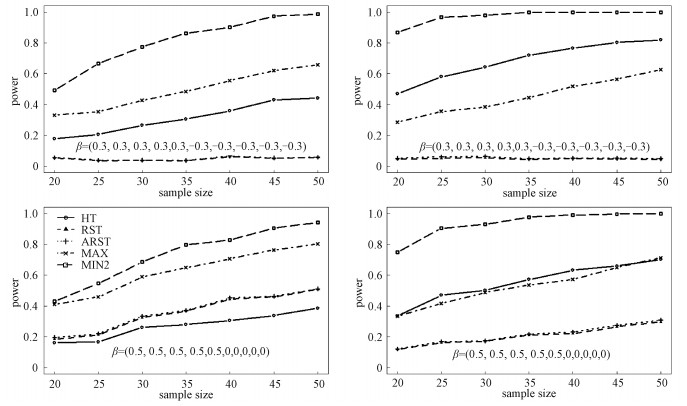
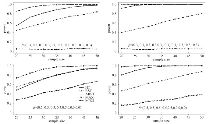
(a) β=(0.3, 0.3, 0.3, 0.3, 0.3, -0.3, -0.3, -0.3, -0.3, -0.3)^T;

(b) β=(0.5, 0.5, 0.5, 0.5, 0.5, 0, 0, 0, 0, 0)^T.

The results for Log-normal and Laplace distributions are displayed in Figs. 1 and 2, respectively, with ρ=0.3 on the left panels and ρ=0.7 on the right panels. For scenario (a), we can see that the RST and ARST have smallest powers, which are close to 0.05. It is reasonable since the differences among the outcomes are counteracted. With the increase in the sample size, the powers of HT, MAX, and MIN2 increase. The MIN2 is the most powerful among all the tests. Sometimes, the power increase for MIN2 reaches more than 30% compared with other tests. For example, for Log-normal distribution, when n₁=n₂=30 and ρ=0.3, the empirical powers of HT, RST, ARST, MAX, and MIN2 are 0.266, 0.038, 0.040, 0.427, and 0.775, respectively. When n₁=n₂=30 and ρ=0.7, the empirical powers of HT, RST, ARST, MAX, and MIN2 are 0.643, 0.055, 0.064, 0.384, and 0.980, respectively. For Laplace distribution, the power increase for MIN2 is sometimes more than 10% over other tests. For example, for scenario (b) when n₁=n₂=25 and ρ=0.3, the empirical powers of HT, RST, ARST, MAX, and MIN2 are 0.439, 0.144, 0.151, 0.498, and 0.72, respectively. When n₁=n₂=25 and ρ=0.7, the empirical powers of HT, RST, ARST, MAX, and MIN2 are 0.895, 0.182, 0.190, 0.538, and 0.997, respectively.

Next, we consider the influences of large sample size and dimension on the efficacy of our MIN2. The simulation data are generated from (4), where $\epsilon$ follows Laplace distribution with mean vector 0 and covariance matrix (Δ_ij), where Δ_ii=1 for i∈{1, 2, …, k} and Δ_ij=ρ=0.3(0.7) for i≠j∈{1, 2, …, k}. Here we consider two types of alternative hypotheses:

(c)(β₁=…=β_k/2=0.05, β_k/2+1=…=β_k=-0.05)^T;

(d)(β₁=…=β_k/2=0.1, β_k/2+1=…=β_k=0)^T.

The results are shown in Table 3. It can be seen that the power of MIN2 increases with the sample size when the dimension is fixed. For example, when k=20 and ρ=0.3 under scenario(c), the empirical powers of HT, RST, ARST, MAX, and MIN2 are 0.137, 0.055, 0.054, 0.120, and 0.262 for n₁=n₂=100 and 0.270, 0.052, 0.052, 0.151, and 0.609 for n₁=n₂=200, respectively. Similarly, the power of MIN2 rises drastically with the increment of the dimension relative to other tests when the sample size is fixed. For example, when n₁=n₂=100 and ρ=0.7 under scenario(d), the powers of all the tests are 0.234, 0.088, 0.091, 0.148, and 0.480 for k=10, 0.344, 0.093, 0.092, 0.153, and 0.657 for k=20, and 0.434, 0.105, 0.106, 0.155, and 0.808 for k=30, respectively. So, the performance of our MIN2 is superior to the other tests in the two cases when the sample size or dimension becomes larger.

3 Application

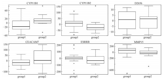
We apply the HT, RST, ARST, MAX, and MIN2 to the data on the aging human brain ^[3]. A total of 30 samples are divided into two groups on account of age. The ages of subjects in group 1 are less than 73 and those in group 2 are larger than 73, where the threshold of 73 is suggested by the authors of Ref.[3]. The aim is to investigate the difference between the two groups with gender as a covariate. Six gene chips (accession number), CYP11B1, CYP11B2, D26561, CEACAM7, ESRRB, and MMP15, are treated as multiple endpoints. Figure 3 shows the box-plots of six gene chips after removing the effect of gender. It is most likely that there exists difference between the two groups. Furthermore, the average values of three gene chips, CY11B1, D26561, and CEACAM7, of group 1 are less than those of group 2, but for the other gene chips, CYP11B2, ESRRB and MMP15, the results are contrary. We carry out the HT, RST, ARST, MAX, and MIN2 to detect the difference between the two groups and the p-values of the above five tests are 0.409, 0.782, 0.794, 0.243, and 0.024, respectively. Evidently, except for MIN2, the other tests fail to detect the difference between the two groups after removing effect of gender at the nominal level of 0.05.

4 Conclusion

Studies involving multiple outcomes are fairly common in many research areas. Many procedures including parametric and nonparametric ones have been developed in the literature without considering covariates. Actually in applications, the auxiliary covariates may often be recorded on each subject. If some covariates are associated with outcomes, the precision may be improved by adjusting for this relationship. In this work, we propose an MIN2 test to compare the difference between two groups for multiple outcomes with covariate adjustment. Through the simulation studies, the MIN2 test controls the type Ⅰ error rate very well and has superior power to other existing nonparametric tests.