In the last decades, various well-known financial models based on the time-homogeneous diffusion processes have arisen. In this work, we are concerned about how to estimate the drift and diffusion coefficients of the processes. We generally consider the time-homogeneous Markov process {X_t} given by the stochastic differential equations

$ {\rm{d}}{X_t} = \mu \left( {{X_t}} \right){\rm{d}}t + \sigma \left( {{X_t}} \right){\rm{d}}{B_t}, $

(1)

where {B_t, t>0} is a standard one-dimensional Brownian motion, and μ(·) and σ(·) are the drift and diffusion coefficients, respectively, dependent on {X_t}. There have been a great amount of studies on parametric methods to estimate μ(·) and σ(·)^{[1, 2, 3]}. One of the major limitations of these methods is that the specific parametric forms of μ(·) and σ(·) have to be assumed first. In order to model more complex drift and diffusion functions and reduce the bias of the estimators, nonparametric regression techniques have been introduced in this area. Florens-Zmirou^[4] first proposed nonparametric estimation with discrete sampling observations for the diffusion term, while the nonparametric kernel estimators of the drift and diffusion functions of a stationary process based on a set of discrete sampling observations were developed by Jiang and Knight^[5].

Stanton^[6] constructed the first-, second-, and third-order approximation formulas for μ(·) and σ(·), in which the unknown conditional expectations estimated by Nadaraya-Watson kernel regression were given, and claimed the superiority of higher-order approximations. By deriving the higher-order approximations and computing the asymptotic variances, Fan and Zhang^[7] concluded that higher-order approximations could reduce the numerical approximation errors of asymptotic biases, but the asymptotic variances would escalate nearly exponentially with the order of approximation. To overcome this difficulty, they adopted the local polynomial techniques to estimate the drift and diffusion functions and applied such techniques to some well-known short-term interest rate models. It turned out that this approach might produce the negative results for the diffusion functions when the higher-order approximations were used. To ensure the nonnegativity of the diffusion functions, Ziegelmann^[8] and Yu and Jones^[9] proposed positive nonparametric conditional variance estimators and Xu^[10] proposed reweighted functional estimation of the diffusion coefficient based on reweighting the conventional Nadaraya-Watson estimator. In addition, Yu et al.^[11] developed the log P-splines and local log-linear method to semiparametrically estimate a class of time-inhomogeneous diffusion processes. Due to the heavy reliance on the logarithmic transformation of the diffusion function, which brings additional bias term, the method is not asymptotically equivalent to the local linear estimator.

In this work, we make use of B-spline basis functions to estimate the drift and diffusion functions based on higher-order approximations, and compare it with the local polynomial techniques. Our simulation results show that the B-spline method indeed outperforms the local polynomial method.

1 The estimators of the drift and diffusion functions

We introduce the estimators of the drift and diffusion functions based on higher-order approximations^[7]. Given a time-homogeneous diffusion process {X_t} satisfying (0.1) and an arbitrary n+1 order continuous differentiable function f(·), the conditional expected increment can be expressed as

$ \begin{array}{*{20}{c}} {E\left[{\left. {f\left( {{X_{t + \mathit{\Delta } }}} \right)-f\left( {{X_t}} \right)} \right|{X_t}} \right] = {\cal L}f\left( {{X_t}} \right)\mathit{\Delta } + }\\ {\frac{1}{2}{{\cal L}^2}f\left( {{X_t}} \right){\mathit{\Delta } ^2} + \cdots + \frac{1}{{n!}}{{\cal L}^n}f\left( {{X_t}} \right){\mathit{\Delta } ^n} + O\left( {{\mathit{\Delta } ^{n + 1}}} \right), } \end{array} $

(2)

where the infinitesimal generator ${\cal L} $ of the process {X_t} is defined as

$ {\cal L}f\left( x \right) = f'\left( x \right)\mu \left( x \right) + \frac{1}{2}f''\left( x \right){\sigma ^2}\left( x \right). $

(3)

Setting f(x)=x-X_t and (x-X_t)² in (3), we have ${\cal L} $f(x)=μ(X_t) and ${\cal L} $f(x)=σ²(X_t).

Furthermore, we rewrite (2) at the different time steps jΔ, j=1, …, k, and get a kth-order approximation scheme

$ \frac{1}{\mathit{\Delta } }\sum\limits_{j = 1}^k {{a_{k, j}}E\left[{f\left( {{X_{t + j\mathit{\Delta } }}} \right)-f\left( {{X_t}} \right)\left| {{X_t}} \right.} \right]} \approx {\cal L}f\left( {{X_t}} \right) $

(4)

with the approximation error (-1)$ ^{k + 1}\frac{{{{\cal L}^{k + 1}}f\left( {{X_t}} \right)}}{{\left( {k + 1} \right)}}{\Delta ^k} + O\left( {{\Delta ^{k + 1}}} \right)$, where ${a_{k, j}} = {\left( {-1} \right)^{j + 1}}\left( \begin{array}{l} k\\ j \end{array} \right)/j, j = 1, \cdots, k $ (see Ref.[7] for details). Setting f(x)=x-X_t and (x-X_t)² in (4), we reach the kth-order approximation schemes of μ(·) and σ²(·)

$ \begin{array}{*{20}{c}} {\mu \left( {{X_t}} \right) = \frac{1}{\mathit{\Delta } }\sum\limits_{j = 1}^k {{a_{k, j}}E\left( {{X_{t + j\mathit{\Delta } }} - {X_t}\left| {{X_t}} \right.} \right)} + O\left( {{\mathit{\Delta } ^k}} \right), }\\ {{\sigma ^2}\left( {{X_t}} \right) = \frac{1}{\mathit{\Delta } }\sum\limits_{j = 1}^k {{a_{k, j}}E\left( {{{\left( {{X_{t + j\mathit{\Delta } }} - {X_t}} \right)}^2}\left| {{X_t}} \right.} \right)} + }\\ {O\left( {{\mathit{\Delta } ^k}} \right).} \end{array} $

(5)

2 B-spline techniques

Fan and Zhang^[7] proposed the qth-degree (q≥0) local polynomial techniques for estimating the conditional expectations in (5), and computed the asymptotic variances of nonparametric estimators. In this section, we will adopt B-spline techniques to estimate μ(·) and σ²(·).

2.1 Estimation for μ(·) using B-Spline

Our goal is to obtain the smooth function μ(x)=E(Y_iΔ|X_iΔ). To this end, we fit the discrete (n-k) pairs of synthetic data (X_iΔ, Y_iΔ), X_iΔ∈[α, β], i=1, …, n-k by the model Y_iΔ=μ(X_iΔ)+ε_i, where ${Y_{i\mathit{\Delta }}} = \frac{1}{\mathit{\Delta }}\sum\limits_{j = 1}^k {{a_{k, j}}\left( {{X_{\left( {i + j} \right)\mathit{\Delta }}}-{X_{i\mathit{\Delta }}}} \right)} $. Let p₁ be the order of the B-spline and define a sequence of knots α=x₁=x₂=…=x_p1 < x_p1+1 < … < x_p1+J1+1=x_p1+J1+2=…=x_2p1+J1=β on an interval [α, β]. Then μ(x) can be expanded in terms of B-spline basis functions as μ(x)=B₁(x)a, where a=(a₁, …, a_m1)′, B₁(x)=(B₁(x), …, B_m1(x)), m₁=J₁+p₁, and B_j(x) is defined as

$ {B_{j, 1}}\left( x \right) = \left\{ \begin{array}{l} 1, \;\;\;\;{x_j} < \cdots < {x_{j + 1}}\\ 0, \;\;\;\;{\rm{otherwise}}{\rm{.}} \end{array} \right. $

$ \begin{array}{*{20}{c}} {{B_{j, p1}}\left( x \right) = \frac{{x - {x_j}}}{{{x_{j + {p_1} - 1}} - {x_j}}}{B_{j, {p_1} - 1}}\left( x \right) + }\\ {\frac{{{x_{j + {p_1}}} - x}}{{{x_{j + {p_1}}} - {x_{j + 1}}}}{B_{j + 1, {p_1} - 1}}\left( x \right), } \end{array} $

for j=1, …, m₁ (the convention x/0=0 is used). When p₁ is chosen as the order of B-spline basis functions, B_j(x)=B_{j, p1}(x), j=1, …, m₁ for the simplicity.

To avoid the excessively "wiggly" estimated curve $ \hat \mu \left( x \right)$, we take the roughness penalty a′R₁a into account^[12]. Then the coefficients a_j can be obtained by minimizing

$ {\rm{PENSSE}}\left( {\rm{a}} \right) = {\left( {\mathit{\boldsymbol{Y}} - {\mathit{\boldsymbol{H}}_1}\mathit{\boldsymbol{a}}} \right)^\prime }\left( {\mathit{\boldsymbol{Y}} - {\mathit{\boldsymbol{H}}_1}\mathit{\boldsymbol{a}}} \right) + {\lambda _1}\mathit{\boldsymbol{a'}}{\mathit{\boldsymbol{R}}_1}\mathit{\boldsymbol{a}}, $

(6)

where Y=(Y_1Δ, …, Y_(n-k)Δ)′, R₁=$\int {{D^2}{\mathit{\boldsymbol{B}}_1}\left( x \right){D^2}\mathit{\boldsymbol{B}}{'_1}\left( x \right){\rm{d}}x}, {\mathit{\boldsymbol{H}}_1} = \left( {{\mathit{\boldsymbol{B}}_1}\left( {{X_{1\mathit{\Delta }}}} \right), \cdots, {\mathit{\boldsymbol{B}}_1}\left( {{X_{\left( {n-k} \right)\mathit{\Delta }}}} \right)} \right)' $, D² is the second-order differential operator, λ₁ is the smoothing parameter which controls the smoothness of a fitted curve.

In this work, we choose the best value of λ₁ by minimizing GCV(λ₁)(generalized cross-validation)

$ {\rm{GCV}}\left( {{\lambda _1}} \right) = \frac{{{\rm{RS}}S\left( {{\lambda _1}} \right)}}{{{{\left\{ {1 - {{\left( {n - k} \right)}^{ - 1}}{\rm{tr}}\left( {{\mathit{\boldsymbol{S}}_{{\lambda _1}}}} \right)} \right\}}^2}}}, $

where RSS$\left( {{\lambda _1}} \right) = \left( {\mathit{\boldsymbol{Y}}-{\mathit{\boldsymbol{H}}_1}\mathit{\boldsymbol{\hat a}}} \right)'\left( {\mathit{\boldsymbol{Y}}-{\mathit{\boldsymbol{H}}_1}\mathit{\boldsymbol{\hat a}}} \right) $ is the residual sum of squares and the smoother matrix of S_λ1=H₁(H′₁H₁+λ₁R₁)^-1H′₁, tr(S_λ1) is the trace of S_λ1. By minimizing (2.8), we get the penalized B-spline regression estimator of the vector of coefficients $\mathit{\boldsymbol{\hat a}} = {\left( {\mathit{\boldsymbol{H}}{'_1}{\mathit{\boldsymbol{H}}_1} + {\lambda _1}{\mathit{\boldsymbol{R}}_1}} \right)^{-1}}\mathit{\boldsymbol{H}}'\mathit{\boldsymbol{Y}} $, and furthermore reach the estimator for the drift function

$ \hat \mu \left( x \right) = {\mathit{\boldsymbol{B}}_1}\left( x \right)\mathit{\boldsymbol{\hat a}} + {\mathit{\boldsymbol{B}}_1}\left( x \right){\left( {{{\mathit{\boldsymbol{H'}}}_1}{\mathit{\boldsymbol{H}}_1} + {\lambda _1}{\mathit{\boldsymbol{R}}_1}} \right)^{ - 1}}{{\mathit{\boldsymbol{H'}}}_1}\mathit{\boldsymbol{Y}}. $

(7)

2.2 Estimation for σ²(·) using B-spline with nonnegative restrictions

Similarly, the square of diffusion function σ²(x) can be also expressed as a linear combination of the B-splines B_j(x) in the form σ²(x)=B₂(x)c, where c=(c₁, …, c_m2), B₂(x)=(B₁(x), …, B_m2(x)), m₂=J₂+p₂, J₂ and p₂ are the numbers of interval knots and the order of B-spline, respectively. In order to ensure the positivity of σ²(x), we impose the reasonable constraint c_j≥0, (j=1, …, m₂) due to the property of the coefficients c_j of B-spline B_j(x) that there are no more sign changes in σ²(x) than those in the sequence c_j.

Under the constraint c≥0, the estimation of c can be achieved by the following optimization problem with a linear inequality constraint

$ \begin{array}{*{20}{c}} {{\rm{minimise}} \to {{\left( {\mathit{\boldsymbol{Z}} - {\mathit{\boldsymbol{H}}_2}\mathit{\boldsymbol{c}}} \right)}^\prime }\left( {\mathit{\boldsymbol{Z}} - {\mathit{\boldsymbol{H}}_2}\mathit{\boldsymbol{c}}} \right) + {\lambda _2}\mathit{\boldsymbol{c'}}{\mathit{\boldsymbol{R}}_2}\mathit{\boldsymbol{c}}}\\ {{\rm{with}}\;\mathit{\boldsymbol{c}} \ge 0, } \end{array} $

(8)

where Z=(Z_1Δ, …, Z_(n-k)Δ)′, Z_iΔ=$ \frac{1}{\mathit{\Delta }}{\sum\limits_{j = 1}^k {{a_{k, j}}\left( {{X_{\left( {i + j} \right)\mathit{\Delta }}}-{X_{i\mathit{\Delta }}}} \right)} ^2}$$, i = 1, \cdots, n-k, {\mathit{\boldsymbol{R}}_2} = \int {{D^2}{\mathit{\boldsymbol{B}}_2}\left( x \right){D^2}\mathit{\boldsymbol{B}}{'_2}\left( x \right){\rm{d}}x} $, and ${\mathit{\boldsymbol{H}}_2} = \left( {{\mathit{\boldsymbol{B}}_2}\left( {{Z_{1\mathit{\Delta }}}} \right), \cdots, {\mathit{\boldsymbol{B}}_2}\left( {{Z_{\left( {n-k} \right)\mathit{\Delta }}}} \right)} \right)' $,

The smoothing parameter λ₂ can be chosen by minimizing GCV(λ₂),

$ {\rm{GCV}}\left( {{\lambda _2}} \right) = \frac{{{\rm{RS}}S\left( {{\lambda _2}} \right)}}{{{{\left\{ {1 - {{\left( {n - k} \right)}^{ - 1}}{\rm{tr}}\left( {{\mathit{\boldsymbol{S}}_{{\lambda _2}}}} \right)} \right\}}^2}}}, $

where RSS(λ₂)=$\left( {\mathit{\boldsymbol{Z}}-{\mathit{\boldsymbol{H}}_2}\mathit{\boldsymbol{\hat c}}} \right)'\left( {\mathit{\boldsymbol{Z}}-{\mathit{\boldsymbol{H}}_2}\mathit{\boldsymbol{\hat c}}} \right) $ is the residual sum of squares, ${\mathit{\boldsymbol{\hat c}}} $ is the estimator of c, and the smoother matrix S_λ2=H₂(H′₂H₂+λ₂R₂)^-1H′₂, and tr(S_λ2) is the trace of S_λ2.

2.3 Choosing the order k of approximation

According to the view of Stanton^[6], the approximations to the drift and diffusion functions converge pointwise to μ(·) and σ(·) at a rate Δ^k, and the first-order approximation performs well when the data are sampled weekly or more frequently. However, as the frequency of data decreases, the approximation error of the first-order approximation increases. In order to reduce asymptotic bias of the approximation error, Fan and Zhang^[7] proposed higher-order approximation method. However, the asymptotic variances of such approximations escalate nearly exponentially with the approximations order.

In this work, we balance the asymptotic bias and variance by choosing k=1 for the data sampled weekly or more frequently and opting for the second-order approximation when the sampling frequency decreases or the data over a small range of values.

2.4 Selection of the number of knots and order p

Ruppert^[13] pointed out that the number of the interval knots was not so crucial as the penalty parameter λ. When the chosen number of knot is enough to fit the feature of data, any increase in J will have little effect on the fitting result. Moreover, the computation time will increase as J rises. As a trade-off, Yoshimoto et al.^[14] proposed the statistical criterion BIC to select a suitable J. Apart from BIC statistical criterion, one might use a simple default value. In Ref.[13], Matt Wand suggested that min([$ \frac{{n-k}}{4}$], 35) interval knots were chosen ([x] is the integral part of x), where n is the number of observations, and k is the order of approximation.

To simplify the computation, we set J₁=J₂=min([$\frac{{n-k}}{4} $], 35) and choose equally spaced knots. This turns out not to affect the results. Other choices of the number of knots have also been tried, and similar results display.

As for the selection of p, we choose p₁=p₂=4. The reason for such selection is that the simulation results show the order 4 B-splines fit the drift and diffusion functions well enough and the higher order spline functions will increase the computation, which overwhelms the approximation precision.

3 Simulation

In this section, we apply our proposed method to three examples. Then we compare our method with local polynomial method. To assess the performance of the two estimation methods, we use the following two measures^[15].

Measure 1  Mean absolute deviation error

$ {\rm{MADE}}\left( {\hat \sigma _t^2} \right) = {m^{ - 1}}\sum\limits_{i = 1}^m {\left| {{Z_{i\mathit{\Delta } }} - \hat \sigma _i^2} \right|}, $

Measure 2  Ideal mean absolute deviation error

$ {\rm{IMADE}}\left( {\hat \sigma _t^2} \right) = {m^{ - 1}}\sum\limits_{i = 1}^m {\left| {\hat \sigma _i^2 - \sigma _i^2} \right|}, $

where m is the length of the testing sample, $ {{\hat \sigma }_i}$ is the estimation of the volatility, and σ_i is the true. These measures are used to assess the performance of different procedures for estimating the volatility. However, for the real data analysis, Measure 2 is not applicable. For the drift function, these measures can also be employed.

3.1 Cox-ingersoll-ross squared-root(CIR SR) model

In this example, we consider the well-known CIR SR model

$ {\rm{d}}{X_t} = \left( {\alpha + \beta {X_t}} \right){\rm{d}}t + \sigma X_t^{1/2}{\rm{d}}{B_t}, t \ge {t_0}, $

(9)

where {X_t} is a measurable Markov process. B_t is a standard Brownian motion. Our simulation data are generated by using the discrete time order 1.0 strong approximation scheme (see Ref.[16] for details) as follows:

$ \begin{array}{l} {X_{{t_{i + 1}}}} \approx {X_{{t_i}}} + \left[ {\alpha + \beta {X_{{t_i}}} - {4^{ - 1}}{\sigma ^2}} \right]{\mathit\Delta } + \\ \;\;\;\;\;\;{2^{ - 1}}\sigma \left\{ {\left[ {{X_{{t_i}}} + \left( {\alpha + \beta {X_{{t_i}}} - {4^{ - 1}}{\sigma ^2}} \right){\mathit\Delta } + } \right.} \right.\\ \;\;\;\;\;\;\left. {\left. {\sigma \left( {{X_{{t_i}}}} \right)_ + ^{1/2}{\varepsilon _i}\sqrt {\mathit\Delta } } \right]_ + ^{1/2} + \left( {{X_{{t_i}}}} \right)_ + ^{1/2}} \right\}{\varepsilon _i}\sqrt {\mathit\Delta } ,\\ \;\;\;\;\;\;\;\;\;\;\;\;\;{\rm{for}}\;i = 1, \cdots ,n - 1, \end{array} $

(10)

where {ε_i}_i=1^n-1 are independent and standard normal variables, x₊=max(x, 0), the time points t₁ < … < t_n, are equally spaced, and Δ is the step size.

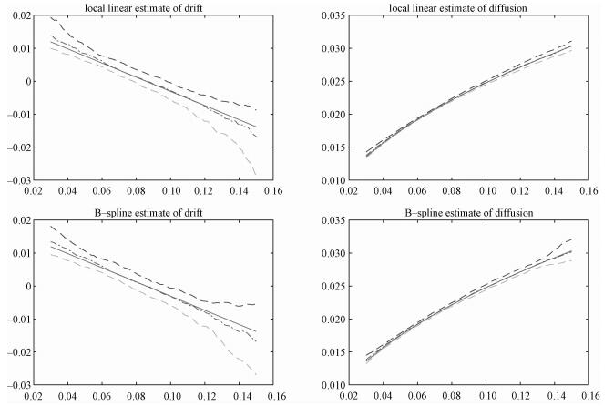
In order to compare with local polynomial techniques, we adopt the same values of model parameters for simulation: α=0.018 392 5, β=-0.214 59, σ=0.078 30, and Δ=1/52. To begin with, a sample path of length 5 000 is generated by the discretization scheme (10) and setting the initial value X₀=0.1, where the first 4 500 observations are in-sample data and the remaining 500 observations out-sample data. Then the estimators of the drift and diffusion functions are calculated respectively through kth-order approximation. Here we choose k=1, as the simulation data are weekly ones. For the purpose of comparison, we simulate 100 sample paths with range interval =[0.03, 0.15], and set the number of interval knots J₁=J₂=35 on the interval . The simulation results are presented in Fig. 1 and Table 1.

In this example, smoothing parameters λ₁ and λ₂ are chosen as 1×10^-3 and 1×10^-4 by minimizing GCV(λ₁) and GCV(λ₂), respectively. The bandwidth parameter for the local linear estimation is generated from the rule

$ h = C \times {\rm{std}}\left( {{X_\mathit{\Delta } }, \cdots, {X_{\left( {n - k} \right)\mathit{\Delta } }}} \right){n^{ - 1/5}}, $

(11)

where C=6. In Table 1 it is shown that the B-spline method possesses certain superior performance because of its lower MADE and IMADE.

3.2 Geometric Brownian motion (GBM) model

We consider another familiar example of geometric Brownian motion determined by

$ {\rm{d}}{X_t} = \left( {\mu + \frac{1}{2}{\sigma ^2}} \right){X_t}{\rm{d}}t + \sigma {X_t}{\rm{d}}{B_t}, t \ge {t_0}, $

(12)

where B_t is a standard one-dimensional Brownian motion. The used parameter values are the same as these in Ref.[7]. μ=0.087, σ=0.178, and the state value X₀=1, Δ=1/250, h=2×std(X_Δ, …, X_(n-k)Δ)n^-1/5. Using these values and following the order 1.0 scheme, we generate 1 000 sample paths of length 1 000 observations,

$ \begin{array}{*{20}{c}} {{X_{{t_{i + 1}}}} \approx {X_{{t_i}}} + \left( {\mu + {2^{ - 1}}{\sigma ^2}} \right){X_{{t_i}}}{\mathit\Delta } + \sigma {X_{{t_i}}}{\varepsilon _i}\sqrt {\mathit\Delta } + }\\ {{2^{ - 1}}{\sigma ^2}{X_{{t_i}}}\left( {\varepsilon _i^2 - 1} \right){\mathit\Delta } .} \end{array} $

(13)

For each simulation, we set the first 900 observations as in-sample data and the remaining observations as out-sample data. In this example, smoothing parameters λ₁=0.01 and λ₂=0.005. Other parameters are the same as these in subsection 3.1. The results are summarized in Table 2.

3.3 Verifying the nonnegativity of diffusion function

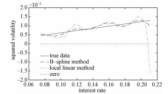
In this part, we generate 600 observations from model (9), and use the first 500 observations as in-sample observations and the remaining as out-sample observations. The simulation data set is presented in Fig. 2(a). Stanton^[6] proposed that the first-order approximation had a bad performance over a small range of values or when the sampling frequency decreased. In order to illustrate that the local polynomial techniques are not suitable for the higher-order approximations, we use the second-order approximation to estimate the squared volatility and set h=0.016, λ₂=1×10^-5. In Fig. 2(b) we display the discrete points of second-order approximation of squared volatility, many of which are negative.The results are shown in Fig. 3 and Table 3. It is seen in Fig. 3 that the fitting results of the squared volatility have negative values at the right boundary when we use the local polynomial method.

This example shows that the restricted B-spline method not only has a lower MADE and IMADE, but also guarantees the nonnegativity of the volatility which is shown in Fig. 3.

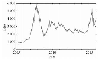
4 Application 4.1 Application of the B-spline techniques to HS300 index

To understand the dynamics of the stock market of China, we apply our proposed techniques to the HS300 index data. The data consist of 2 610 daily observations from 8 April 2005 to 31 December 2015, and are presented in Fig. 4.

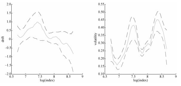
Because the data are the daily ones, the first-order approximation is a good choice in the light of the estimation effect and variance inflation. Following the conventional practice in finance research, we first take the logarithmic transformation of the price index and then obtain the range interval =[6.706 9, 8.678 8]. We set the number of equally spaced interval knots J₁=J₂=35. By using the rule proposed in section 2, smoothing parameters λ₁=0.1 and λ₂=0.02 are chosen. The estimation results of drift and volatility are presented in Fig. 5. The solid curves are the estimation, and the dashed curves are the 95% bootstrap confidence intervals.

Regression bootstrap technique is used to calculate the bootstrap confidence intervals (see Ref[17] for details). We denote S_ti=X_ti+1-X_ti for the original HS300 data {X_ti, i=1, …, n}, and then generate the bootstrap responses {S_ti^*} using $ S_{{t_i}}^* = \hat \mu \left( {{X_{{t_i}}}} \right)\mathit{\Delta} + \hat \sigma \left( {{X_{{t_i}}}} \right){\sqrt {\mathit\Delta }}\varepsilon _i^*, i = 1, \cdots, n-1$, where the bootstrap residuals {ε_i^*, i=1, …, n-1} are sampled randomly with replacement from $\left\{ {{{\hat \varepsilon }_i}, i = 1, \cdots, .n-1} \right\} $ and $ {{\hat \varepsilon }_i} = \frac{{{S_{{t_i}}}-\hat \mu \left( {{X_{{t_i}}}} \right)\mathit{\Delta }}}{{\hat \sigma \left( {{X_{{t_i}}}} \right){\sqrt {\mathit\Delta }}}}$. It is easy to obtain the bootstrap samples $\left\{ {\left( {{X_{{t_i}}}, Y_{i\mathit{\boldsymbol{ \boldsymbol{\varDelta} }}}^*} \right)_{i = 1}^{n-1}} \right\} $ and $\left\{ {\left( {{X_{{t_i}}}, Z_{i\mathit{\boldsymbol{ \boldsymbol{\varDelta} }}}^*} \right)_{i = 1}^{n-1}} \right\} $ when the first-order approximation is used. If a higher-order approximation is involved, we just need to set X^*_t1=X_t1, and then generate a regression bootstrap sample {X^*_ti, i=1, …, n}. Similarly, the bootstrap sample $\left\{ {\left( {{X_{{t_i}}}, Y_{i\mathit{\boldsymbol{ \boldsymbol{\varDelta} }}}^*} \right)_{i = 1}^{n-1}} \right\} $ and $ \left\{ {\left( {{X_{{t_i}}}, Z_{i\mathit{\boldsymbol{ \boldsymbol{\varDelta} }}}^*} \right)_{i = 1}^{n-1}} \right\}$ can be obtained. In our studies, the bootstrap confidence intervals are calculated based on 1 000 bootstrap samples.

4.2 Treasury bond case study

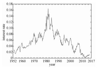
We apply the two techniques proposed above to the three-year treasury bond from the secondary market rates on the last trading day of each month and compare the estimation effects of squared volatility between the two methods. The data set contains 753 monthly observations from 30 April 1953 to 31 December 2015, and is presented in Fig. 6.

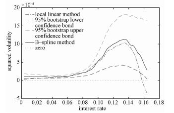
Here we use the second-order approximation to estimate the squared volatility of model (1) for the monthly three-year treasury bond data. The estimation of squared volatility with the 95% bootstrap confidence bond based on 1 000 bootstrap samples by the penalized B-spline with nonnegative restriction techniques is displayed in Fig. 7 (the solid curve). In Fig. 7 the dashed-dotted curve denotes the estimation obtained by local polynomial techniques. It is obvious that the squared volatility estimated by local polynomial techniques with h=0.028 9 is negative when the treasury bond rate is equal to 0.16. This result shows that the fitting effect of penalized B-spline with nonnegative restriction techniques is better than that of the local polynomial. Such effect will be very obvious when the higher-order approximation is used. In this study, we choose =[0.003 0, 0.164 5], J₂=35, and λ₂=1×10^-5.

5 Conclusion

The B-spline method gives a good performance for the drift and volatility estimation. When a higher-order approximation is adopted, the B-spline method is a better choice because it not only has lower MADE and IMADE but also guarantees the nonnegativity of the volatility, while the local polynomial method does not. Our techniques will be extended to time-inhomogeneous diffusion models in the future.