In many practical applications, high-resolution (HR) images are often desired in many practical applications such as video surveillance, biometrics identification, medical imaging, and so on. However, due to the limitations of physical imaging devices, the images we observe are not always at a desired resolution level. The apparent aliasing effects often seen in digital images are caused by the limited number of charge-coupled device (CCD) pixels used in digital device. Using denser CCD arrays (with smaller pixel size) not only increases the cost but also adds more noises^[1]. Moreover, there are many low-resolution (LR) valuable images and available videos. The goal of super-resolution (SR) is to recover a high-resolution image from one or a few low-resolution images.

In the SR literature, SR approaches are classified into three groups: interpolation-based methods^[2-4], regularization-based methods^[5-6] and example-based methods^[7-10].

Interpolation-based methods upscale the size of an LR image by estimating the pixels in the HR grids via a base function^{[2, 4]} or interpolation kernel^[3]. This kind of method always performs well in low-frequency areas (smooth areas) but it cannot recover high-frequency areas (edge) because it often blurs image along edges.

Regularization-based methods assume that the high-frequency information lost in an LR image is split across multiple LR images with sub-pixel misalignments. There are many different priors used in these methods, e.g. nonlocal means (NLM)^[6] and total-variation (TV)^[5]. However, in practical applications, it is hard to obtain these previous priors. Moreover, if HR images are computed by simulating the image formation process, these approaches are limited^[11].

In example learning-based SR methods, the local patches in the desired HR image and those in the input LR image are assumed to admit a sparse approximation over the same dictionary learned from the HR and LR database. The missing HR pixels can be learnt from low-resolution and high-resolution pairs of examples in the database. Freeman et al.^[7] first proposed a relation model between LR image patches and corresponding HR image patches by using the Markov network. Yang et al.^[8] created a database which combines LR image patches with HR image patches and used sparse coding to reconstruct HR images. Based on an observation that natural images tend to contain repetitive visual content, Glasner et al.^[9] proposed a super resolution method from a single image. Li et al.^[10] proposed a single image super-resolution reconstruction method, which was based on global non-zero gradient penalty and non-local Laplacian sparse coding.

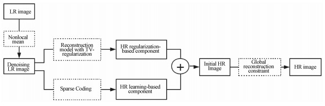
1 Our proposed approach

In this study, we propose a novel approach based on nonlocal means, total variation-regularization, and sparse coding. The overall framework of the proposed approach is shown in Fig. 1. As shown in Fig. 1, firstly, LR image is denoised by using nonlocal means (NLM)^[6] which preserves geometric structure well. This denoised LR image is used twice to produce two components in initial HR image. The regularization-based component is obtained from a reconstruction model with total variation-regularization. The regularization-based component maintains part of the sharpness of the edges and some details. Meanwhile, the HR learning-based componentis reconstructed by exploring the sparse coding which explores the co-occurrence relationship between LR training patches and their corresponding HR high-frequency patches. Finally, the global reconstruction constraint is applied to the initial image for making the final HR image natural.

1.1 Regularization-based component reconstruction

In practical applications, the real images are always noisy. In this study, we use noisy LR image as the input to adapt to real-world conditions. During the regularization-based component reconstruction, LR image is denoised and upscaled.

1.1.1 Denoising by nonlocal means

We use NLM to denoise the noisy LR image. This approach assumes that image content tends to repeat itself within some similar neighborhoods among natural images. Therefore, the similar patches found in other locations provides more information of the target patch. By averaging all similar patches in the neighborhoods, the target patch is denoised^{[6, 12]}.

The target patch is calculated by

$x\left( {k,l} \right) = \frac{{\sum {_{\left( {i,j} \right) \in N\left( {k,l} \right)}w\left[ {k,l,i,j} \right]y\left( {i,j} \right)} }}{{\sum {_{\left( {i,j} \right) \in N\left( {k,l} \right)}w\left[ {k,l,i,j} \right]} }},$

(1)

where N(k, l) stands for the neighborhood of the pixel (k, l) in the input image and the term w[k, l, i, j] is the weight for the (i, j)-th neighborhood pixel of pixel (k, l). The input pixels are y(i, j), and the pixel value of output image in (k, l) is x(k, l).

The weights w[k, l, i, j] for each pixel are computed based on both radiometric (gray-level) proximity and geometric proximity between the pixels, namely

$\begin{array}{l} w\left[ {i,j,k,l} \right] = f\left( {\sqrt {{{\left( {k - i} \right)}^2} + {{\left( {l - j} \right)}^2}} } \right) \cdot \exp \\ \left\{ { - \frac{{\sum\limits_{m = - q}^q {\sum\limits_{n = - q}^q {{{\left[ {y\left( {k + m,l + n} \right) - y\left( {i + m,j + n} \right)} \right]}^2}} } }}{{2\sigma _r^2}}} \right\}, \end{array}$

(2)

where the former function f takes the geometric distance into account and is monotonically non-increasing. It may take many forms such as a Gaussian, a box function, a constant, and others. The latter computes the Euclidean distance between two image patches centered around two involved pixels. The size of these patches is $\left( {2q + 1} \right) \times \left( {2q + 1} \right)$. The parameter ${\sigma _r}$ controls the effect of the grey-level difference between the two pixels.

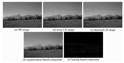
After NLM, the output LR image preserves many low-frequencies and some high-frequencies of input LR image. Besides, the output LR image is denoised. Figure 2 (c) shows the denoised LR image of "meadow" image.

1.1.2 Reconstruction model with total variation-regularization

The output image of the previous step should be upscaled to satisfy the demand.

For single image SR problem, the image generation process of an LR image from HR image is defined as

$\boldsymbol{Y} = \boldsymbol{DHX} + \varepsilon ,$

(3)

where X and Y are the HR and LR images, respectively, which are rearranged in lexicographic order. D is the decimation operation, H represents the blurring operation, and ε is the system noise which is always assumed as Gaussian noise^[13].

Solving (3) is an ill-posed problem^[14]. There exists an infinite number of solutions which satisfy (3). Therefore, regularization is a useful method to produce a stable solution. Besides, regularization improves the rate of convergence.

A regularization term is usually implemented as a penalty factor. One of the most successful regularization methods for denoising and deblurring is the total-variation (TV) method^[15]. The TV criterion penalizes the total amount of change in the image as measured by the L₁ norm of the magnitude of the gradient. Then the regularizing function becomes

$\boldsymbol{\widehat X} = \arg \;\mathop {\min }\limits_X \left\| {\boldsymbol{DHX} - \boldsymbol{Y}} \right\|_2^2 + \lambda {\left\| {\nabla \boldsymbol{X}} \right\|_1},$

(4)

where $\lambda $, a global parameter, balances similarity cost against regularization cost. $\nabla $ is the gradient operator.

We use a fast iterative shrinkage/thresholding algorithm (FISTA) to solve this minimization problem^[16]. Figure 2 (d) shows the regularization-based component of "meadow" image.

1.2 Learning-based component reconstruction

Before the learning-based component reconstruction, we need to train several over-complete dictionaries.

1.2.1 design of training databases

Clustering of the training image patch pairs is linked to the effect of dictionary learning. The collected patch pair is HR patch together with LR patch.

Recently, extracting the local geometry structure for the low-resolution image patch in order to boost the prediction accuracy was suggested. There are many filters to extract the edge information such as a high-pass filter^[17], a set of Gaussian derivative filters^[18], the first-order gradients and second-order gradients of the patches^[4]. Here, we use the LR feature patches, which are the first-order gradients and second-order gradients, to replace the original LR patches.

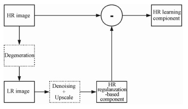
To obtain better HR high-frequency information, we use HR learning (high-frequency) component to replace the original HR patch. HR learning component is obtained in the following steps. Firstly, the HR image is downsampled by the desired factor s and added Gaussian noise as the noisy LR image. Secondly, the denoised LR image is constructed by NLM. Thirdly, the regularization-based component of HR image is constructed by reconstruction model with TV-regularization. Finally, we can obtain the HR learning component by calculating the residual between HR and HR regularization-based component. Figure 1 shows the decomposition process.

Once these training patch pairs are collected, we divide these pairs into different clusters by the dominant direction of LR patch. The patches with similar dominant direction will be collected into one cluster.

1.2.2 Couple dictionary learning

Sparse coding method is to find a sparse representation of one signal in an over-complete dictionary D. The dictionary is usually learned from many training sets $\boldsymbol{X} = \left[ {{x_1}, \cdots ,{x_n}} \right] \in {R^{m \times n}}.\;{\rm{Let}}\;\boldsymbol{D} = \left[ {{d_1}, \cdots {d_k}} \right] \in {R^{m \times k}}$ be the dictionary matrix, and let $S = \left[ {{s_1}, \cdots ,{s_n}} \right] \in {R^{k \times n}}$ be the coefficient matrix. Then, the objective function of sparse coding is

$\begin{array}{c} \arg \;\mathop {\min }\limits_{D,S} \left\{ {\left\| {\boldsymbol{X} - \boldsymbol{DS}} \right\|_F^2 + \alpha {{\left\| \boldsymbol{S} \right\|}_1}} \right\}\\ {\rm{s}}{\rm{.t}}{\rm{.}}\;\;{\left\| {{d_i}} \right\|^2} \le 1,i = 1,2, \cdots ,k, \end{array}$

(5)

where minimizing ${\left\| S \right\|_1}$ is to enforce sparsity, $\left\| {\boldsymbol{X} - \boldsymbol{DS}} \right\|_F^2$ is the empirical loss function, and the parameter $\alpha $ balances fidelity of the approximation to X and sparsity of the solution.

Let the sampled training image patch pair in the j-th cluster be $P = \left\{ {\boldsymbol{X}_h^j,\boldsymbol{Y}_l^j} \right\}$, where $\boldsymbol{X}_h^j = \left\{ {x_1^j,x_2^j, \cdots ,x_n^j} \right\}$ are the set of HR learning component patches and $\boldsymbol{Y}_l^j = \left\{ {y_1^j,y_2^j, \cdots ,y_n^j} \right\}$ are the corresponding LR feature patches. Joint dictionary training method is used to train two coupled dictionaries for each cluster. Similar to the treatment in Reb.[8], the single sparse coding problem in the HR learning component patch and the LR feature patch are

$\boldsymbol{D}_h^j = \arg \mathop {\min }\limits_{\boldsymbol{D}_h^j,S} \left\{ {\left\| {\boldsymbol{X}_h^j - cD_h^jS} \right\|_F^2 + \alpha {{\left\| S \right\|}_1}} \right\},$

(6)

and

$\boldsymbol{D}_l^j = \arg \;\mathop {\min }\limits_{\boldsymbol{D}_l^j,S} \left\{ {\left\| {\boldsymbol{Y}_l^j - \boldsymbol{D}_l^jS} \right\|_F^2 + \alpha {{\left\| \boldsymbol{S} \right\|}_1}} \right\},$

(7)

where D_h^j and D_l^j represent j-th clustera's coupled dictionaries.

In order to force the HR and LR representations to share the same codes, we combine these objectives

$\begin{array}{l} \;\arg \;\mathop {\min }\limits_{D_h^j,D_l^j,S} \left\{ {\frac{1}{{{N_1}}}\left\| {\boldsymbol{X}_h^j - \boldsymbol{D}_h^j\boldsymbol{S}} \right\|_F^2 + } \right.\\ \left. {\frac{1}{{{N_2}}}\left\| {\boldsymbol{Y}_l^j - \boldsymbol{D}_l^j\boldsymbol{S}} \right\|_F^2 + \alpha \left( {\frac{1}{{{N_1}}} + \frac{1}{{{N_2}}}} \right){{\left\| \boldsymbol{S} \right\|}_1}} \right\}, \end{array}$

(8)

where N₁ and N₂ are the dimensions of the HR learning component and LR feature patch in vector form, respectively. Here, $\frac{1}{{{N_1}}}{\rm{and}}\frac{1}{{{N_2}}}$ balance the two cost terms of (6) and (7). By (6) and (7), (8) can be rewritten as

$\;\;\;\arg \;\mathop {\min }\limits_{D_c^j,S} \left\{ {\left\| {\boldsymbol{B}_c^j - \boldsymbol{D}_c^j\boldsymbol{S}} \right\|_F^2 + \widehat \alpha {{\left\| \boldsymbol{S} \right\|}_1}} \right\},$

(9)

where

$\begin{array}{l} \boldsymbol{B}_c^j = {\left[ {\frac{1}{{\sqrt {{N_1}} }}\boldsymbol{X}_h^j,\frac{1}{{\sqrt {{N_2}} }}\boldsymbol{Y}_l^j} \right]^{\rm{T}}},\\ \boldsymbol{D}_c^j = {\left[ {\frac{1}{{\sqrt {{N_1}} }}\boldsymbol{D}_h^j,\frac{1}{{\sqrt {{N_2}} }}\boldsymbol{D}_l^j} \right]^{\rm{T}}},\\ \widehat \alpha = \alpha \left( {\frac{1}{{\sqrt {{N_1}} }} + \frac{1}{{\sqrt {{N_2}} }}} \right). \end{array}$

For a given test LR image, which is set as the denoise LR image in our method, we sample patches with overlap and extract four features of these patches. Then, for each feature patch y_i, we adaptively select coupled dictionaries D_h^j and D_l^j from all coupled dictionaries, by computing the dominant orientation of y_i to find the most similar cluster. We compute the sparse coefficient s_i under the proper dictionary D_l^j, and we can obtain the HR patch estimation ${\boldsymbol{X}^{j*}} = \boldsymbol{D}_h^j{s_i}$. The whole HR learning component is reconstructed by averaging all the reconstructed patches such as X^j*. Figure. 2 (e) shows the learning-based component of "meadow" image. Then the initial HR image X₀ is obtained by adding the reconstructed component and the learning component.

1.3 The global reconstruction constraint

Unexpected artifacts are always found in the initial HR image X₀ because of the simple addition operation. Considering the image generation process of an LR image from HR image, we find the closest image to X₀ which satisfies the image generation process

${\boldsymbol{X}^*} = \arg \;\mathop {\min }\limits_X \left\{ {\left\| {\boldsymbol{DHX} - \boldsymbol{Y}} \right\|_2^2 + c\left\| {\boldsymbol{X} - {\boldsymbol{X}_0}} \right\|_2^2} \right\},$

(10)

where c is regularization parament, X^* is the final HR image, and Y is set as the denoised image.

2 Experiments

In our experiments, we perform eleven test images to measure our proposed method by magnifying them two times. All the images come from the Berkeley Segmentation Dataset^[19]①.

http://www.eecs.berkeley.edu/Research/Projects/CS/vision/grouping.

2.1 Experimental configuration

The noisy LR image is produced by artificially adding Gaussian noise to original LR image. The standard deviation of Gaussian noise is set to be 10. We denote it as σ.

In (1) and (2), the research zone N(k, l) is limited to a square neighborhood of 21 pixels×21 pixels. $q = 1.\sigma _r^2 = 4\sigma $. The function f is set to be constant, so that it gives no preference to adjacent patches over distant ones. This makes f more robust to various motion patterns.

In (3), the blurring operation H is set to be an identity matrix.

In (4), global parameter λ is set to be 0.001 and Y is chosen as the denoised LR image.

In (5), parameter α is set to be 0.15.

During the design of training databases, we have trained 12 clusters in total. For each cluster, the coupled dictionaries are trained from 50 000 patch pairs randomly sampled from 100 training images. The sizes of original LR training patch and the corresponding HR patch are set to be 25(5×5) and 100(10×10), respectively. So the LR feature patches which are the first-and second-order gradients of original LR training patch are set to be 100(5×5×4). Considering computation cost and image quality, the dictionary size is always fixed at 512.

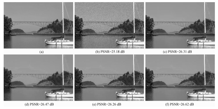
2.2 Results

For showing the effectivity of our proposed method, we use different methods to magnify the 'Boat' image two times in Fig. 2. Figure 4(a) is the original HR image, Figs. 4(b) to 4(e) are the mages solved by using other methods, and Fig. 4(f) is the final HR image by using our method. The input noisy LR image is produced by the generation process in (3). To be convenient to calculate PSNR, we firstly upscale LR image by bicubic interpolation to fix the size of HR image.(See Figs. 4(b) and 4(c)). However, Figs. 4(d), 4(e), and 4(f)retain the same size as in Fig. 4(a).

It is obvious that Fig. 4(b) is very noisy. After denoising Fig. 4(b) by NLM, a smooth image in Fig. 4(c) is obtained and its PSNR value also increases. Figure 4(d) is obtained by using (4) and Y is set as in Fig. 4(c). Figure 4(e) is the initial HR image which has been described in Fig. 1. Figure 4(f) is the final result by using (10) to optimize the initial image. It is easy to see that the final image in Fig. 4(f) is most similar to the original HR image in Fig. 4(a).

To certify the validity of our method, we deal with eleven images as same as (b)-(f) in Fig. 2. We show the PSNR results in Table 1.

In Table 1, it is obvious that original noisy LR image always gives the worst performance because of the noteworthy noise. The denoised image achieves better results than original noisy LR image, which indicates that denoising is effective. Because of unexpected artifacts, the PSNR of initial HR image is often smaller than that of the regularization-based component. By using the global reconstruction constraint, these artifacts are eliminated and the PSNR always increases.

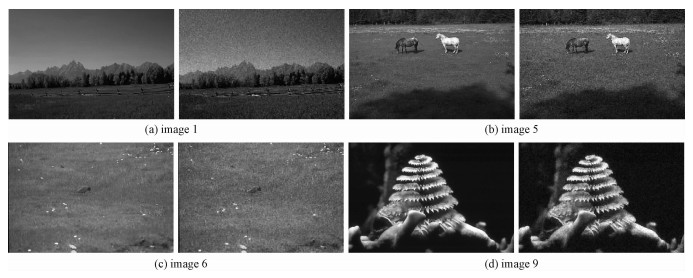
The regularization-based component sometimesachieves the best performance. Figure 5 lists these images. Among these images, the important high-frequency information is destroyed by noise. When we try to recovery high-frequency information from the noisy LR image, it is hard to distinguish the true information from noise. The learning-base component has a low confidence so that the regularization-based component without the learning-base component achieves the best result.

3 Conclusion

In this study, we propose a new approach based on regularization-based component and learning-based component. We apply the global reconstruction to make the images natural. As the input image is noisy, we denoise image firstly by nonlocal means. Then the reconstruction-based component is obtained by reconstruction model with total variation-regularization. The learning-based component is produced by sparse coding and the initial HR image is obtained by adding the reconstructed component and the learning component. However, the initial HR image always looks unnatural. Hence, the global reconstruction constraint is used.

Experimental results demonstrate the effectiveness and robustness of the proposed approach.