 2016, Vol. 33


Consider the numerical approximations for stochastic differential equations (SDEs) in the Itô sense as follows
| $\left\{ \begin{align} & dX=a\left( t,X \right)dt+b\left( t,X \right)dW\left( t \right), \\ & X\left( {{t}_{0}} \right)={{X}_{0}}, \\ \end{align} \right.$ | (1) |
where X,a(t,x1,…,xn),b(t,x1,…,xn) are n-dimensional column-vectors and W(t) is a standard Wiener process. In addition,we suppose that the coefficients a(t,x1,…,xn) and b(t,x1,…,xn) are sufficiently smooth functions that guarantee the existence and the uniqueness of the solution in the interval [t0,t0+T](see Refs.[1-2] for details). Let X(t;t0,x,ω),t0≤t≤t0+T, be the solution of the SDE (1) where ω is an elementary event. Moreover,we denote by Xk,k=0,…,N,tk+1-tk=h,tN=t0+T, the numerical method for (1) based on the one-step approximation X=X(t+h;t,x).
As is known in Refs.[3-6],there are many kinds of numerical schemes for the SDE (1). However,the construction of these approximations are usually based on the SDEs in the Itô sense. Hence,it is meaningful to investigate whether we could construct the methods by using their equivalent SDEs in the sense of Stratonovich and Backward-Itô.
1 Full implicit schemes 1.1 Equivalentequations in the sense of Stratonovich and Backward-Itô
As is known in Refs.[1-2, 5-6],the equivalent equation with respect to the SDE (1) in the sense of Stratonovich is as follows:
| $dX=\left( \left( a-\frac{1}{2}\frac{\partial b}{\partial x}b \right)\left( t,X \right) \right)dt+b\left( t,X \right){}^\circ dW\left( t \right)$ | (2) |
where X(t0)=X0 and
Based on the relationship between the Itô integral and the Stratonovich integral,we can obtain the SDE (2). Analogously,we can define another stochastic integral,Backward-Itô integral,and get the equivalent equation of SDE (1) in the sense of Backward-Itô. Let (Ω,F) be a measure space with the probability P and Ft be the σ-algebra generated by the n-dimensional Brownian motions Bi(s)(1≤i≤n,0≤s≤t). We denote by V(S,T) the class of functions
f(t,ω):[0,∞)×Ω→R,
such that
1) (t,ω)→f(t,ω) is B×F-measurable,where B denotes the Borel σ-algebra on [0,∞);
2) f(t,ω) is Ft-adapted and
Furthermore,let L2(P) be a Hilbert space with the following inner product
(X,Y)L2(P):=E[X·Y];X,Y∈L2(P).
Definition 1.1 Suppose that f∈V(0,T) and t→f(t,ω) is continuous for a.e.ω. Then the Backward-Itô integral of f is defined by
| $\int\limits_{0}^{T}{f\left( t,\omega \right)*dW\left( t \right)}=\underset{h\to 0}{\mathop{\lim }}\,\sum\limits_{j}{f}\left( {{t}_{j+1}},\omega \right)\Delta {{W}_{j}}$ |
whenever the limit exists in L2(P).
Note that this kind of integral has been introduced in Ref.[3]. For convenience,we give it the name Backward-Itô integral. According to the definition of the Backward-Itô integral,we can easily get the relationship between the Itô integral and the Backward-Itô integral as follows:
| $\int\limits_{0}^{T}{f\left( t,\omega \right)*dW\left( t \right)}=\int\limits_{0}^{T}{f\left( t \right)dW\left( t \right)}+\int\limits_{0}^{T}{\frac{\partial f\left( t \right)}{\partial W}}dt,$ | (3) |
where f∈V(0,T) and t→f(t,ω) is continuous for a.e. ω. Then using formula (3),we can obtain the equivalent SDE in the sense of Backward-Itô
| $dX=\left( \left( a-\frac{\partial b}{\partial x}b \right)\left( t,X \right) \right)dt+b\left( t,X \right)*dW\left( t \right),$ | (4) |
where X(t0)=X0.
1.2 The convergence theorem on mean-square methods from Ref.[4]Theorem 1.1 See Ref.[4]. Suppose that the one-step approximation X(t+h;t,x) has the order of accuracy p1 for the mathematical expectation of the deviation and order of accuracy p2 for the mean-square deviation. More precisely,for arbitrary t0≤t≤t0+T-h,x∈Rn the following inequalities hold:
| $\begin{align} & \left| E\left( \left( X-\bar{X} \right)\left( t+h;t,x \right) \right) \right|\le K{{\left( 1+{{\left| x \right|}^{2}} \right)}^{\frac{1}{2}}}{{h}^{{{p}_{1}}}} \\ & {{\left[ E{{\left| \left( X-\bar{X} \right)\left( t+h;t,x \right) \right|}^{2}} \right]}^{\frac{1}{2}}}\le K{{\left( 1+{{\left| x \right|}^{2}} \right)}^{\frac{1}{2}}}{{h}^{{{p}_{2}}}} \\ \end{align}$ | (5) |
Also,let
p2≥12,p1≥p2+12.
Then for any N and k=0,…,N the following inequality holds:
| $\begin{align} & {{\left[ E{{\left| \left( X-\bar{X} \right)\left( {{t}_{k}};{{t}_{0}},{{X}_{0}} \right) \right|}^{2}} \right]}^{\frac{1}{2}}} \\ & \le K{{\left( 1+{{\left| {{X}_{0}} \right|}^{2}} \right)}^{\frac{1}{2}}}{{h}^{{{p}_{2}}-\frac{1}{2}}}, \\ \end{align}$ | (6) |
i.e. the order of accuracy of the method constructed using the one-step approximation X(t+h;t,x) is p=p2-
Theorem 1.2 See Refs.[5-6]. Let the one-step approximation X(t+h;t,x) satisfy the condition of Theorem 2.1. Suppose that
| $\begin{align} & \left| E \right.\left( \bar{X}\left( t+h;t,x \right)-\tilde{X}\left( t+h;t,x \right) \right)=O\left( {{h}^{{{p}_{1}}}} \right), \\ & {{\left[ E{{\left| \bar{X}\left( t+h;t,x \right)-\tilde{X}\left( t+h;t,x \right) \right|}^{2}} \right]}^{\frac{1}{2}}}=O\left( {{h}^{{{p}_{2}}}} \right), \\ \end{align}$ | (7) |
with the same h1p and h2p. Then the method based on the one-step approximation
Besides,the authors of Refs.[4-6] have mentioned that the increments of Wiener processes should be substituted by truncated random variables in implicit schemes. In detail,
| ${{\zeta }_{h}}=\left\{ \begin{align} & \xi ,if\left| \xi \right|\le {{A}_{h}}, \\ & {{A}_{h}},if\xi >{{A}_{h}}, \\ & -{{A}_{h}},if\xi <{{A}_{h}}, \\ \end{align} \right.$ | (8) |
where
implicit schemes
First,we consider the SDE (2). As is known,the exact solution is
| $\begin{align} & X\left( t+h;t,x \right)=x+\int\limits_{t}^{t+h}{b\left( s,X\left( s \right) \right)}\circ dW\left( s \right)+ \\ & \int\limits_{t}^{t+h}{\left[ \left( a-\frac{1}{2}\frac{\partial b}{\partial x}b \right)\left( s,X\left( s \right) \right) \right]}ds, \\ \end{align}$ | (9) |
which coincides with the solution of the SDE (1) by using the Stratonovich integrals. Let the mid-rectangle formula approximate the integrals in (9). We can get a full implicit scheme of the first mean-square order as follows
| $\begin{align} & {{X}_{k+1}}={{X}_{k}}+b\left( {{t}_{k}}+\frac{h}{2},\frac{{{X}_{k}}+{{X}_{k+1}}}{2} \right){{\zeta }_{h}}\sqrt{h}+ \\ & \left[ \left( a-\frac{1}{2}\frac{\partial b}{\partial x}b \right)\left( {{t}_{k}}+\frac{h}{2},\frac{{{X}_{k}}+{{X}_{k+1}}}{2} \right) \right]h. \\ \end{align}$ | (10) |
Similarly,the solution of the SDE (4) is
| $\begin{align} & X\left( t+h;t,x \right)=x+\int\limits_{t}^{t+h}{b\left( s,X\left( s \right) \right)}*dW\left( s \right)+ \\ & \int\limits_{t}^{t+h}{\left[ \left( a-\frac{1}{2}\frac{\partial b}{\partial x}b \right)\left( s,X\left( s \right) \right) \right]}ds, \\ \end{align}$ | (11) |
which is also in agreement with the solution of the SDE (1). Similarly,if the integrals in (11) are approximated by the right-rectangle formula,the numerical scheme has the form:
| ${{X}_{k+1}}={{X}_{k}}+b\left( {{t}_{k}}+h,{{X}_{k+1}} \right){{\zeta }_{h}}\sqrt{h}+\left[ \left( a-\frac{\partial b}{\partial x}b \right)\left( {{t}_{k}}+h,{{X}_{k+1}} \right) \right]h,$ |
which we can prove to be of mean-square order 0.5. However,based on an analog of Taylor expansion of the solution (11),another full implicit method
| $\begin{align} & {{X}_{k+1}}={{X}_{k}}+\left[ \left( a-\frac{1}{2}\frac{\partial b}{\partial x}b \right)\left( {{t}_{k+1}},{{X}_{k+1}} \right) \right]h+ \\ & \left[ \frac{1}{2}\frac{\partial b}{\partial x}b\left( {{t}_{k+1}},{{X}_{k+1}} \right) \right]\zeta _{h}^{2}h+ \\ & b\left( {{t}_{k}},{{X}_{k}} \right){{\zeta }_{h}}\sqrt{h}, \\ \end{align}$ | (12) |
which is of the first mean-square order,could be constructed.
2 Mean-square order of the full implicit schemes
Theorem 2.1 The numerical method (10) with
Proof According to an analog of Taylor expansion of the solution (9),the one-step approximation X(t+h;t,x) as follows
| $\begin{align} & \bar{X}=x+\left[ \left( a-\frac{1}{2}\frac{\partial b}{\partial x}b \right)\left( t+h,x \right) \right]h+ \\ & b\left( t,x \right)\Delta W\left( h \right)+\frac{1}{2}\frac{\partial b}{\partial x}b\left( t,x \right){{\left( \Delta W\left( h \right) \right)}^{2}}. \\ \end{align}$ | (13) |
has the first mean-square order of convergence under appropriate conditions. The full implicit method (10) we propose is
| $\begin{align} & \tilde{X}=x+\left[ \left( a-\frac{1}{2}\frac{\partial b}{\partial x}b \right)\left( t+\frac{h}{2},\frac{x+\tilde{X}}{2} \right) \right]h+ \\ & b\left( t+\frac{h}{2},\frac{x+\tilde{X}}{2} \right){{\zeta }_{h}}\sqrt{h}. \\ \end{align}$ | (14) |
After expanding the right side of (14) about x,we get
| $\begin{align} & \tilde{X}=x+\left[ \left( a-\frac{1}{2}\frac{\partial b}{\partial x}b \right)\left( t+\frac{h}{2},x \right) \right]h+ \\ & b\left( t,x \right){{\zeta }_{h}}\sqrt{h}+\frac{1}{2}\frac{\partial b}{\partial x}\left( t,x \right)b\left( t,x \right)\zeta _{h}^{2}{{\rho }_{1}}. \\ \end{align}$ | (15) |
It is obvious that |E(ρ1)|=O(h2) and E(ρ1)2=O(h3). Since
| $\begin{align} & \bar{X}-\tilde{X}=b\left( t,x \right)\left( \Delta W\left( h \right)-{{\zeta }_{h}}\sqrt{h} \right)+ \\ & \frac{1}{2}\frac{\partial b}{\partial x}\left( t,x \right)b\left( t,x \right)\left( {{\xi }^{2-}}\zeta _{h}^{2} \right)h-{{\rho }_{1}} \\ \end{align}$ | (16) |
it is possible to show that
| $\begin{align} & E{{\left( \bar{X}-\tilde{X} \right)}^{2}}\le KE{{\left( \xi -{{\zeta }_{h}} \right)}^{2}}+ \\ & K{{h}^{2}}E{{\left( {{\xi }^{2}}-\zeta _{h}^{2} \right)}^{2}}+O\left( {{h}^{3}} \right), \\ \end{align}$ | (17) |
where K is a sufficiently large constant. Using the inequalities E(ξ-ζh)h2=O(h2) and E(ξ2-ζ2)2≤27h in Ref.[7],we can easily prove
Theorem 2.2 The numerical method (12) with
Proof Considering the numerical method (12),we expand the right side of the solution (11) and obtain
| $\begin{align} & X\left( t+h;t,x \right) \\ & =x+\int\limits_{t}^{t+h}{b\left( s,X\left( s \right) \right)}*dW\left( s \right)+ \\ & \int\limits_{t}^{t+h}{\left[ \left( a-\frac{\partial b}{\partial x}b \right)\left( s,X\left( s \right) \right) \right]}ds, \\ & =x+\left[ \left( a-\frac{\partial b}{\partial x}b \right)\left( t,x \right) \right]h+b\left( t,x \right)\Delta W\left( h \right)+ \\ & \int\limits_{t}^{t+h}{\int_{t}^{s}{Lb}\left( \theta ,X\left( \theta \right) \right)}d\theta *dW\left( s \right)+ \\ & \int\limits_{t}^{t+h}{\int_{t}^{s}{\frac{\partial b}{\partial x}}b\left( \theta ,X\left( \theta \right) \right)}dW\theta *dW\left( s \right)+{{\rho }^{1}} \\ & =x+\left[ \left( a-\frac{\partial b}{\partial x}b \right)\left( t,x \right) \right]h+b\left( t,x \right)\Delta W\left( h \right)+ \\ & \int\limits_{t}^{t+h}{\int_{t}^{s}{\frac{\partial b}{\partial x}}b\left( t,x \right)}dW\theta *dW\left( s \right)+{{\rho }^{2}}, \\ \end{align}$ | (18) |
where |E(ρ1)|=O(h2),E(ρ1)2=O(h3),|E(ρ2)|=O(h2), and E(ρ2)2=O(h3). Since
| $\begin{align} & X\left( t+h;t,x \right) \\ & =x+\left[ \left( a-\frac{\partial b}{\partial x}b \right)\left( t,x \right) \right]h+ \\ & \frac{1}{2}\frac{\partial b}{\partial x}b\left( t,x \right){{\left( \Delta W\left( h \right) \right)}^{2}}+\frac{1}{2}\frac{\partial b}{\partial x}b\left( t,x \right)h+ \\ & b\left( t,x \right)\Delta W\left( h \right)+{{\rho }^{3}} \\ & =x+\left[ \left( a-\frac{1}{2}\frac{\partial b}{\partial x}b \right)\left( t+h,X \right) \right]h+ \\ & \frac{1}{2}\frac{\partial b}{\partial x}b\left( t+h,X \right){{\left( \Delta W\left( h \right) \right)}^{2}}+ \\ & b\left( t,x \right)\Delta W\left( h \right){{\rho }^{4}} \\ \end{align}$ | (19) |
where |E(ρ3)|=O(h2),E(ρ3)2=O(h3),|E(ρ4)|=O(h2), and E(ρ4)2=O(h3). However,the increments of the Wiener processes in (19) should be substituted by truncated random variables. Finally,by using Theorem 2.1,we prove the theorem. □
3 Numerical testExample Consider the stochastic differential equation
| $dX=tX\left( t \right)dW\left( t \right),X\left( 0 \right)={{X}_{0}}$ | (20) |
whose exact solution is
| $X\left( t \right)={{X}_{0}}\exp \left( \frac{1}{2}\int\limits_{0}^{t}{{{s}^{2}}}ds+\int\limits_{0}^{t}{sdW\left( s \right)} \right).$ |
In application to (20),the Euler Method reads
| ${{X}_{n+1}}={{X}_{n}}+{{t}_{n}}{{X}_{n}}\Delta {{W}_{n}},$ | (21) |
and the two full implicit methods we proposed have the forms
| $\begin{align} & {{X}_{n+1}}={{X}_{n}}-\frac{h}{4}\left( {{t}_{n}}+\frac{h}{2} \right)\left( {{X}_{n}}+{{X}_{n+1}} \right)+ \\ & \frac{1}{2}\left( {{t}_{n}}+\frac{h}{2} \right)\left( {{X}_{n}}+{{X}_{n+1}} \right){{\zeta }_{h}}\sqrt{h} \\ \end{align}$ | (22) |
and
| $\begin{align} & {{X}_{n+1}}={{X}_{n}}-\frac{h}{2}{{\left( {{t}_{n}}+h \right)}^{2}}{{X}_{n+1}}+ \\ & {{t}_{n}}{{X}_{n}}{{\zeta }_{h}}\sqrt{h}+\frac{1}{2}{{\left( {{t}_{n}}+h \right)}^{2}}{{X}_{n+1}}\zeta _{h}^{2}, \\ \end{align}$ | (23) |
which are of the first mean-square order.
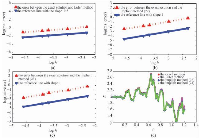
The numerical tests examine the behaviors of the numerical methods in two aspects: the sample trajectories produced by the numerical methods and the true solution shown in Fig. 1(d) and the convergence rates of the numerical methods shown in Fig. 1(a),1(b),and 1(c).

|
Download:
|
| Fig. 1 Numerical test of the example | |
Figures 1(a),1(b),and 1(c) show that,comparing with the reference line,the Euler method is of mean-square order 0.5 and the numerical methods (22) and (23) are of the first mean square order. In our experiments we take t=1,X0=10, and h=[0.01,0.02,0.025,0.05,0.1].
Figure 1(d) presents that the numerical approximations (22) and (23) are much closer to the exact solution than the Euler method for X0=2 and h=0.04 within the time interval 0≤t≤1.2.
| [1] | Mao X R. Stochastic differential equations and applications[M]. 2nd ed. Horwood Publishing Limited, 2007 . |
| [2] | Øksendal B. Stochastic differential equations[M]. 6th ed. Springer, 2003 . |
| [3] | Kloeden P E, Platen E. Numerical solution of stochastic differential equations[M]. Berlin Heidelberg: Springer-Verlag, 1992 . |
| [4] | Milstein G N, Tretyakov M V. Stochastic numerics for mathematical physics[M]. Berlin Heidelberg: Springer-Verlag, 2004 . |
| [5] | Milstein G N, Repin Y M, Tretyakov M V. Symplectic integration of Hamiltonian systems with additive noise[J]. SIAM J Numer Anal , 2002, 39 :2066–2088. DOI:10.1137/S0036142901387440 |
| [6] | Milstein G N, Repin Y M, Tretyakov M V. Numerical methods for stochastic systems preserving symplectic structure[J]. SIAM J Numer Anal , 2002, 40 :1583–1604. DOI:10.1137/S0036142901395588 |
| [7] | Deng J, Anton C A, Wong Y S. High-order symplectic schemes for stochastic Hamiltonian systems[J]. Commun Comput Phys , 2014, 16 (1) :169–200. DOI:10.4208/cicp.311012.191113a |