 2016, Vol. 33


2. University of Chinese Academy of Sciences, Beijing 100190, China
2. 中国科学院大学, 北京 100190
SAR repeat-pass interferometry, a mapping mode of InSAR, is a coherent imaging method. The repeat-pass InSAR system uses a single antenna to collect the complex reflectivity of the illuminated scene at different times. By interfering the two images which are made of the same scene in close geometries, it is possible in such a way to cancel the scene reflectivity common to both and to recover the image-domain phase data. When the terrain elevation is still between the two SAR images of an interferometric pair, the deformation over the time interval can be transduced from phase terms. The change between two-pass collections performs sensitive to the phase, so the deformation detecting accuracy afforded is quite exceptional. It is widely used in terrain motion mapping, such as seismic displacement, volcanic motion, glacier drift, and urban subsidence monitoring[1-2].
As the radar resolution increases and its swath widens, the number of observation of multichannel InSAR substantially increases, as well as the complexity of the system. As a result, the tremendous data bring great pressure to the finite storage onboard and down-link data rate. When there is a little deformation among the scenes, the reflectivity data processed by traditional matched filtering method actually becomes compressible.
Sparse microwave imaging[3] is the interdisciplinary of sparse signal processing and microwave imaging technology. Compared with the traditional radar imaging methods based on matched filter theory, sparse microwave imaging algorithms such as compressed sensing (CS)[4-5] could make use of fewer measurements far below the Nyquist Sampling rate to reconstruct the sparse target scene by solving an lq(0<q≤1) norm optimization problem[6-7]. It is convenient for data acquisition, storage, transmission and processing, and it can also reduce the system complexity and achieve high resolution microwave imaging.
Distributed compressed sensing (DCS) based on CS and distributed source coding (DSC) theory is introduced to recover the signals from independent observations of multiple sensors[8-9]. According to the different sparsity assumptions regarding the common and innovation components, three joint sparsity models (JSMs) are proposed in different situations[9]. In the first model, each signal contains a common component that is sparse and an innovation component that is also sparse. In the second model, all signals share the same locations of the nonzero coefficients. In the third model, no signal is itself sparse, yet each signal contains a sparse innovation component so that there still exists a joint sparsity among the signals. In the repeated measurements of SAR, if the observed scenes are sparse themselves or in a transform domain and the echoes are coherent with each other, DCS is applicable to recover the observed scene. If the scenes and their changes are sparse, the joint sparsity of the multiple scenes is lower than a summation of each scenes sparsity. DCS is used extensively in multi-channel SAR imaging[10], moving target detection[11-12], and polarimetric SAR tomography[13].
The main contribution of this paper is the proposal of a model of repeat-pass InSAR combined with DCS in order to detect deformation. Then we conduct a series of ground-based SAR experiments to compare the recovery performance using different algorithms. As a result, taking advantage of the coherence and joint sparsity among multiple scene echoes, the DCS joint observation system can achieve scene reconstruction and deformation detection accurately with fewer observations and lower hardware complexity than CS.
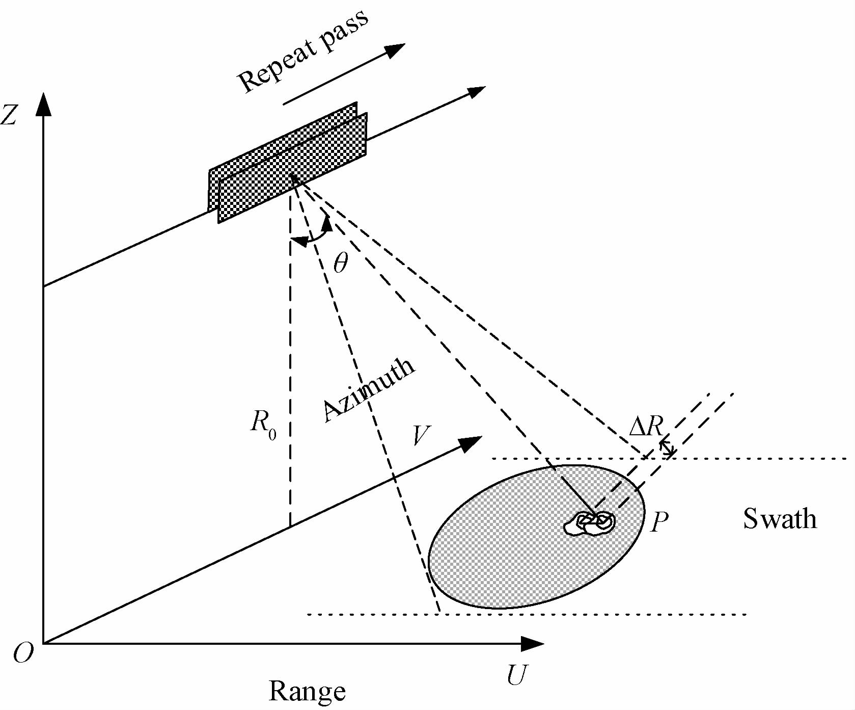
1 Repeat-pass InSAR model overviewRepeat-pass InSAR model[1-2] could illuminate the area and collect the images through azimuth synthetic aperture movement at different time instances using the same platform. Owing to the effects of larger separations in space and time between the image collections and to the fact that the precise orientation of the antenna phase centers is not rigidly fixed, repeat-pass data processing is complicated. In this paper, we would not discuss the impact of these problems and errors in the deformation detecting model. The strip-map imaging geometry model is shown in Fig. 1. The U-axis is the range direction; the V-axis is the flight direction; and the Z-axis is the height dimension. va and H are the platform velocity and height relative to the ground, respectively. The incident angle of emitted waves is θ. ΔR is a small change of the target scene on the slant plane.

|
Download:
|
| Fig. 1 Repeat-pass InSAR geometry model | |
Interferometric processing is meaningful only as applied to images formed from distinct phase histories, where the inter-image differences are functions of quantities we wish to measure. Following a registration, the two complex images from SAR echoes can be formulated as
| $\begin{align} & {{S}_{1}}({{R}_{1}})=\sum i, j{{x}_{1}}({{u}_{i}}, {{v}_{j}})\times ~{{e}^{j4\pi \lambda {{R}_{1}}({{u}_{i}}, {{v}_{j}})}}={{x}_{1}}\times {{e}^{j4\pi \lambda {{R}_{1}}}}, \\ & {{S}_{2}}({{R}_{2}})=\sum i, j{{x}_{2}}({{u}_{i}}, {{v}_{j}})\times {{e}^{j4\pi }}\lambda {{R}_{2}}({{u}_{i}}, {{v}_{j}})={{x}_{2}}\times {{e}^{j4\pi }}\lambda {{R}_{2}} \\ \end{align}$ | (1) |
where R1 and R2 are the distances between the antenna and the target scene in two-pass observations, x1 and x2 are the complex reflectivity of the illuminated scene, and λ is the wave length. If the target scene is close to the vehicle such as ground-based SAR near range imaging, we cannot ignore the attenuation of electromagnetic waves with distance[14]. The phase of the complex images are expressed as
| $\begin{align} & {{\varphi }_{1}}({{R}_{1}})=4\pi \lambda {{R}_{1}}+arg({{x}_{1}}), \\ & {{\varphi }_{2}}({{R}_{2}})=4\pi \lambda {{R}_{2}}+arg({{x}_{2}}) \\ \end{align}$ | (2) |
where arg(x1) and arg(x2) are the phases of x1 and x2, The phase difference is explicitly derived from interferometric processing
| $\begin{align} & {{S}_{1}}({{R}_{1}}){{S}_{2}}{{({{R}_{2}})}^{*}}={{x}_{1}}\cdot {{x}_{2}}\times {{e}^{j4\pi }}\lambda ({{R}_{1}}{{R}_{2}})\times \\ & {{e}^{arg\left( {{x}_{1}} \right)arg({{x}_{2}})}}. \\ \end{align}$ | (3) |
Supposing that arg(x1) is equal to arg(x2), phase shift are defined as
| ${{\varphi }_{1}}{{\varphi }_{2}}=j\frac{4\pi }{\lambda }\Delta R+k\cdot 2\pi , \text{ }k=0, \pm 1, \pm 2, \cdots .$ | (4) |
After phase unwrapping, the real phase can be used to compute ΔR along the slant range.
2 CS and DCS theory review 2.1 CS theoryCS theory[4] can exactly recover a signal, which has sparse supports in one basis, from a small number of projections onto another basis which is incoherent with the first through tractable recovery procedures. The recovery procedures are described as a linear equation given by
| $y=\Phi x+w$ | (5) |
where Φ∈RM×N is the measurement matrix with M<N, y∈RM×1 is the measurement vector, x∈RN×1 is a K-sparse signal of length N, and w∈RN×1 is the additive noise. If the signal x has a sparse representation in a transform domain Ψ given by
| $x=\sum\limits_{i=1}^{N}{{{\psi }_{i}}{{\alpha }_{i}}}=\Psi \alpha $ | (6) |
where α∈RN×1. Substitutlon of the above expression into (5) forms
| $y=\Phi \Psi \alpha +w.$ | (7) |
If the measurement matrix satisfies the restricted isometric property (RIP) or other certain constraint conditions, x can be reconstructed from M=O(Klog(N/K)) measurements by solving an optimiz-ation problem
| $min\|x{{\|}_{1}}s.t.~\|y\Phi \Psi \alpha {{\|}_{2}}\le \varepsilon $ | (8) |
where ε measures the error from the system noise.
2.2 DCS theoryDCS theory[8-9] extends to reconstruct a set of signals, which have sparse representation in their respective domain and are independently observed from multiple sensors. xg∈RN×1 which denotes the g-th (g=1, …, G) signal is coherent with each other, and it can be recovered by
| ${{y}_{g}}={{\Phi }_{g}}{{x}_{g}}+{{w}_{g}}, $ | (9) |
where yg∈RM×1 and Φg∈RM×N are the measure-ment vector and the matrix of the g-th sensor, respectively.
In the first model of DCS, all signals share a common sparse component and each individual signal contains a sparse innovation component expressed as
| ${{x}_{g}}={{z}_{c}}+{{z}_{g}}\text{ }g=1, 2, \ldots , G$ | (10) |
where zc∈RN×1 is the common sparse component and zg∈RN×1 is the innovation component. If they have sparse representations in a transform domain Ψ, we denote them by zc=Ψσc, ‖σc‖0=Kc and zg=Ψσg, ‖σg‖0=Kg. We can deduce a joint sparsity model form expressed as
| $Y=\tilde{\Phi }Z+W$ | (11) |
where Y is the joint measurement vector,
| $$\eqalign{ & Y = \left[ {\matrix{ {{y_1}} \cr \matrix{ {y_2} \hfill \cr \vdots \hfill \cr} \cr {{y_3}} \cr } } \right], Z = \left[ {\matrix{ {{z_c}} \cr \matrix{ {z_1} \hfill \cr \vdots \hfill \cr} \cr {{z_G}} \cr } } \right], W = \left[ \matrix{ {w_1} \hfill \cr {w_2} \hfill \cr \vdots \hfill \cr {w_G} \hfill \cr} \right], \cr & \Phi = \left[ {\matrix{ {{\Phi _1}} & {{\Phi _1}} & 0 & \cdots & 0 \cr {{\Phi _2}} & 0 & {{\Phi _2}} & \cdots & 0 \cr \vdots & \vdots & \vdots & {} & \vdots \cr {{\Phi _G}} & 0 & \cdots & \cdots & {{\Phi _G}} \cr } } \right] \cr} $$ | (12) |
Consequently, DCS can further reduce the total measurements than CS due to the joint sparsity and coherence of all signals.
3 Repeat-pass InSAR joint observ-ation model based on DCSIn this section, we develop a systematic framework of demonstrating the repeat-pass InSAR joint observation model based on DCS. The radar transmits chirp signals, which can be formulated as
| $s\left( t \right)=p\left( t \right){{e}^{j2\pi {{f}_{c}}t}}, $ | (13) |
where
| ${{r}_{g}}\left( t \right)={{\int }_{{{x}_{g}}\in C}}{{x}_{g}}\cdot {{e}^{j2\pi {{f}_{c}}\tau }}({{x}_{g}})p(t\tau ({{x}_{g}}))d{{x}_{g}}+{{w}_{g}}\left( t \right), $ | (14) |
where xg is the reflectivity of the target scene, τ(xg) is the time delay of the echo from the transmitter to the receiver, and wg(t) is the noise of the system receiver.
By discretizing the backscattering coefficient vector of the target scene, the equivalent equation can be expressed as
| ${{y}_{g}}\left( m \right)=\sum\limits_{n=1}^{N}{{{x}_{g}}}\left( n \right)\cdot {{e}^{j2\pi {{f}_{c}}\tau }}_{g}\left( n \right)p(t\left( m \right){{\tau }_{g}}\left( n \right))+{{w}_{g}}\left( t\left( m \right) \right), $ | (15) |
where n=1, 2, …, N, N is the discrete element position of the target scene, xg(n) is the reflectivity in position n, t(m) is the sampling time, τg(n) is the time delay in position n, and wg(t(m))is the additive noise including the system noise and quantization noise.
Denote φg(m, n)=e-j2πfcτg(n)·p(t(m)-τg(n)).Equation (15) can be expressed as
| ${{y}_{g}}\left( m \right)=\sum\limits_{n=1}^{N}{{{x}_{g}}}\left( n \right)\cdot {{\varphi }_{g}}\left( m, n \right)+{{w}_{g}}\left( m \right).$ | (16) |
We will use the following notations for the g-th independent observation model. yg∈CMg×1 is regarded as the g-th echo data with Mg measurements, Φg∈CM×N is the measurement matrix generated by the system parameters, xg is K-sparse, and wg∈CN×1 is the additive noise vector. These symbols are defined as
| $\begin{align} & {{y}_{g}}=\left( \begin{matrix} {{y}_{g}}\left( 1 \right) \\ {{y}_{g}}\left( 2 \right) \\ {{y}_{g}}\left( M \right) \\ \end{matrix} \right), {{x}_{g}}=\left( \begin{matrix} {{x}_{g}}\left( 1 \right) \\ {{x}_{g}}\left( 2 \right) \\ {{x}_{g}}\left( M \right) \\ \end{matrix} \right), {{w}_{g}}=\left( \begin{matrix} {{w}_{g}}\left( 1 \right) \\ {{w}_{g}}\left( 2 \right) \\ {{w}_{g}}\left( M \right) \\ \end{matrix} \right), \\ & {{\Phi }_{g}}=\left( \begin{matrix} {{\Phi }_{g}}\left( 1, 1 \right) & {{\Phi }_{g}}\left( 1, 2 \right) & \cdots & {{\Phi }_{g}}\left( 1, N \right) \\ {{\Phi }_{g}}\left( 2, 1 \right) & {{\Phi }_{g}}\left( 2, 2 \right) & \cdots & {{\Phi }_{g}}\left( 2, N \right) \\ \vdots & \vdots & \vdots & \vdots \\ {{\Phi }_{g}}\left( M, 1 \right) & {{\Phi }_{g}}\left( M, 2 \right) & \cdots & {{\Phi }_{g}}\left( M, N \right) \\ \end{matrix} \right). \\ \end{align}$ | (17) |
Each dependent measurement model can be expressed in a simplified form of
| ${{y}_{g}}={{\Phi }_{g}}\cdot {{x}_{g}}+{{w}_{g}}, $ | (18) |
The two-pass DCS joint observation system can be derived from Equations (10), (11), and (18)
| $$\left[ \matrix{ {y_1} \hfill \cr {y_2} \hfill \cr} \right] = \left[ {\matrix{ {{\phi _1}} & {{\phi _1}} & 0 \cr {{\phi _2}} & 0 & {{\phi _2}} \cr } } \right]\left[ {\matrix{ {{z_c}} \cr {{z_1}} \cr {{z_2}} \cr } } \right] + \left[ \matrix{ {w_1} \hfill \cr {w_2} \hfill \cr} \right].$$ | (19) |
This phase shift can be explicitly seen from the following relationship between z1 and z2 without arg(z1) and arg(z2)
| ${{z}_{1}}\cdot {{z}_{2}}^{}={{z}_{1}}\cdot {{z}_{2}}{{e}^{j\frac{4\pi }{\lambda }}}\Delta R.$ | (20) |
Then we can detect the deformation at sub-Nyquist sampling ratio using DCS method.
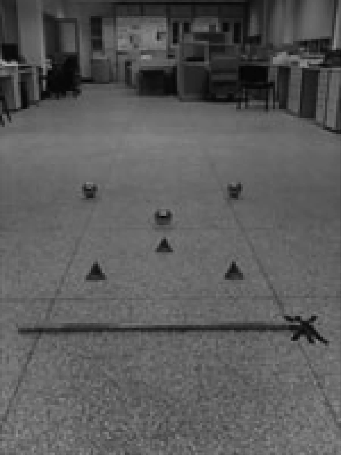
4 Experimental results 4.1 Ground-based SAR imaging resultsWe conduct a series of ground-based SAR experiments to detect deformation of metal targets. Ground-based SAR system uses one antenna to transmit stepped frequency signals and to receive echoes through azimuth synthetic aperture motion along a horizontal straight orbit. By repeat track observation of the target scene at different time, its regional deformation detecting accuracy can attain millimeter. The main propose of the experiments is to compare the performance of deformation detection using different imaging algorithms. The experimental scene is illustrated in Fig. 2.

|
Download:
|
| Fig. 2 Experimental scene | |
There are a 101 cm-long steel, three reflectors, and three metal balls 10 cm in diameter from near to far in the scene, whose spasity is about 5%. The scene is separately observed including common elements and identical elements. We suppose X-axis of the scene is range direction and Y-axis is azimuth. One end of the steel is fixed on the ground and the other end moves 1 cm along positive X-axis directions, between the two observations. The two balls in the distance move 1 cm along positive and negative X-axis directions, respectively. The rest objects are still. The parameters of the ground-based SAR system are given in Table 1.
|
|
Table 1 Ground-based SAR system parameters |
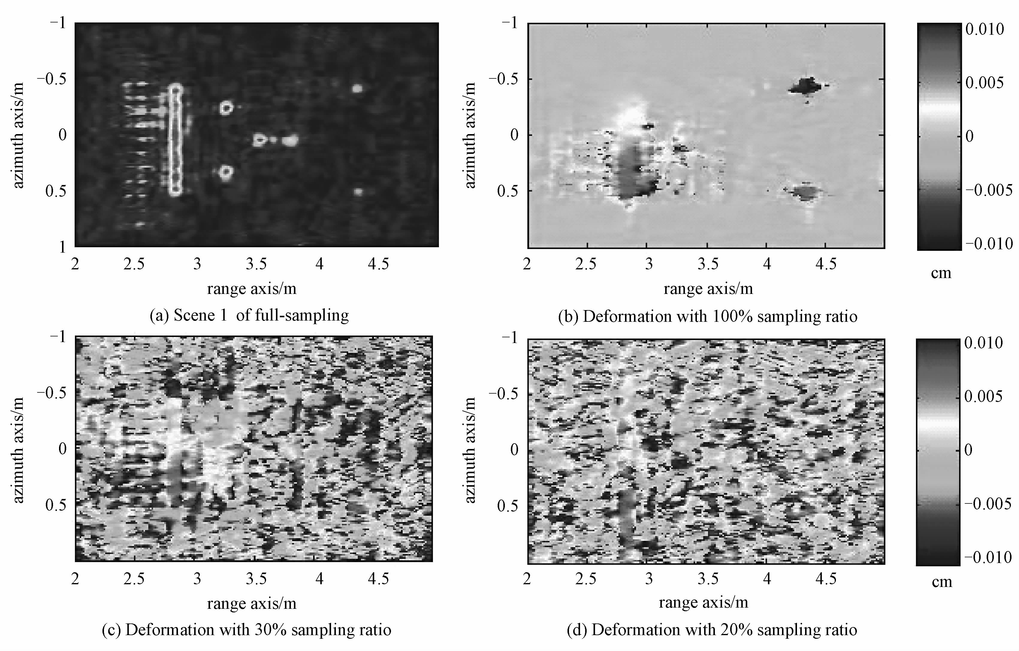
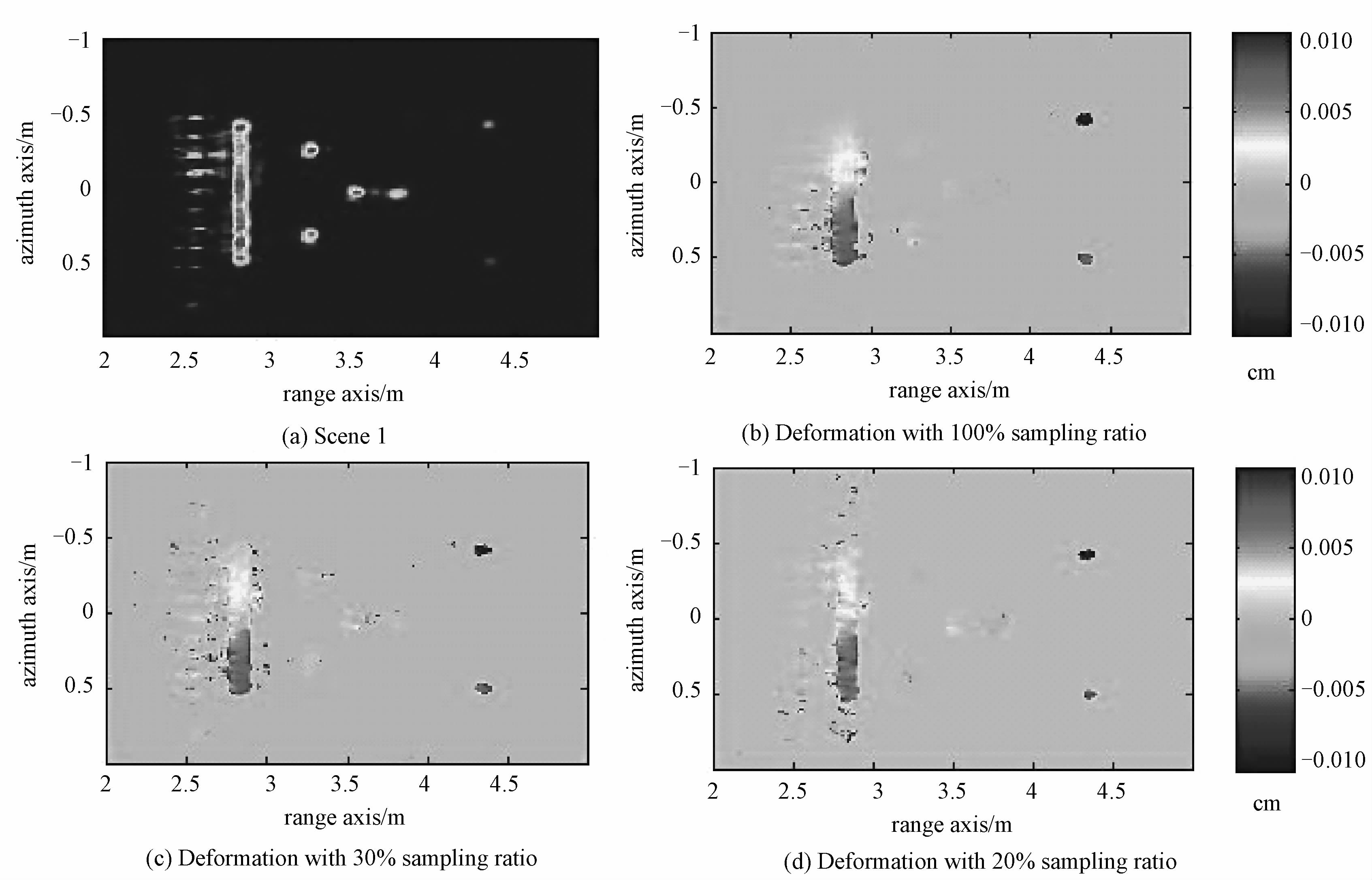
Figure 3 illustrates the imaging results using Omega-k algorithm. How the deformation detecting ability changes has been found with the number of echo samples reducing. The color bars only indicate the deformation of objects in Fig. 3(b), 3(c), and 3(d). Figure 3(a) shows the amplitude image of scene 1 at Nyquist sampling rate in both range and azimuth directions, which is almost similar to scene 2. The metal objects can be distinguished probably and the sidelobes are also included. The gradual displacement of the steel from one end to the other and the two balls apart can be monitored from the phase change of the complex images with full data at Nyquist sampling ratio, as illustrated in Fig. 3(b), in which red part means the positive movement of the targets and blue part means the negative shift. Figure 3(c) and Fig. 3(d) show the deformation images with 30% random sampling ratio (50% of the range data and 60% of the azimuth data) and 20% random sampling ratio(40% of the range data and 50% of the azimuth data), respectively. Sampling ratio reducing can result in aliasing of the targets so that the deformations are unable to distinguish.

|
Download:
|
| Fig. 3 Omega-k imaging results | |
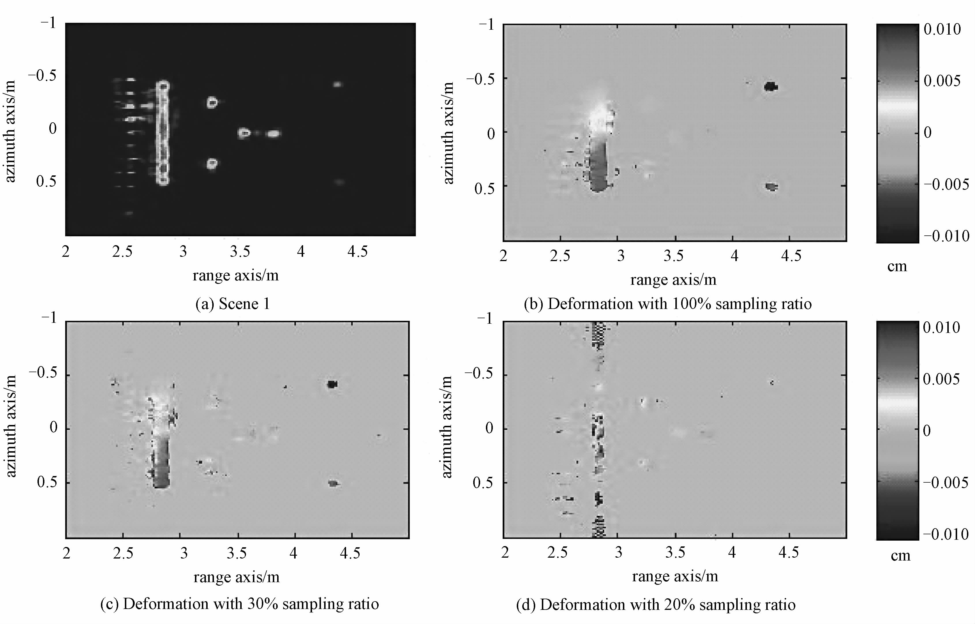
The outcomes via CS imaging algorithm are given in Fig. 4. We can find that the sidelobes of the targets in the amplitude image fade in Fig. 4(a). Figure 4(b) demonstrates that CS algorithm can preserve the phase information of the complex data. The deformation results via CS also have good focus and lower sidelobes so that it is easier to distinguish the movement distribution via CS' than via Omega-k algorithm. When the number of sampling ratio decreases to 30%, the deformation processed by CS between the two scenes can be reconstructed well and aliasing does not appear, as shown in Fig. 4(c). Figure 4(d) shows that the deformation are wrong because the two scenes can not be correctly reconstructed with 20% sampling ratio. Comparing with the matched filtering method, CS recovery algorithm can reduce the number of observations and improve the imagery quality by sidelobes depression. Moreover, deformation detecting performance via CS is much better.

|
Download:
|
| Fig. 4 CS imaging results | |

|
Download:
|
| Fig. 5 DCS imaging results | |
We then use DCS joint imaging algorithm to reconstruct the scenes, as illustrated in Fig. 5. We find that DCS joint processing results have the same features as CS algorithm both in amplitude and phase reconstruction of complex data. The imaging quality and deformation detecting ability is also better than traditional matched filtering methods due to sidelobe depression. See Fig. 5(a), 5(b) and 5(c). When the joint sampling ratio decreases to 20%, the deformation between the two scenes can be reconstructed successfully, as shown in Fig. 5(d). The experiments indicate that the DCS joint observation system can achieve scene reconstruction and deformation detection exactly. It is effective to further reduce independent observations by taking advantage of the coherence and joint sparsity between the multiple scene echoes.
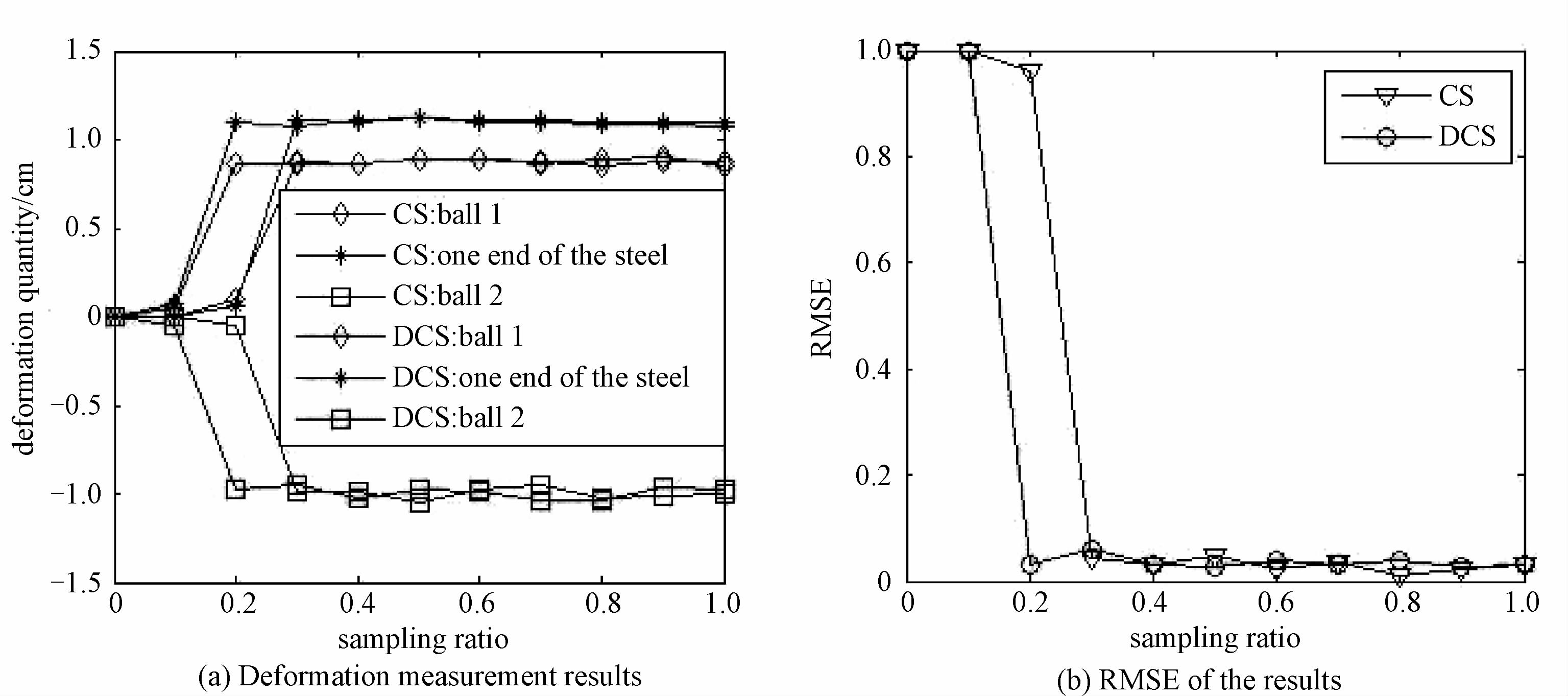
4.2 Deformation error analysisIn order to demonstrate the performance of deformation detecting based on CS and DCS evidently, we calculate the motion of the two balls and the steel from the images with sampling ratio decreasing, shown in Fig. 6(a). Moreover, we use the relative mean square error (RMSE) to measure the deformation error of all the objects. The sampling ratio is supposed to be equal between the two observations. d is the real motion of the objects, and the RMSE is defined as
| $RMSE=E\left( \frac{\left\| \hat{d}-d \right\|_{2}^{2}}{\left\| d \right\|_{2}^{2}} \right), $ | (21) |
where

|
Download:
|
| Fig. 6 Deformation measurements and RMSE analysis in CS and DCS imaging results | |
The measurement error mainly arises from the motion precision rather than the system error. The experimental results agree well with the actual values and the regional deformation detecting accuracy which can attain millimeter. As the sampling ratio is lowering, the DCS joint observation system can still achieve scene recovery and deformation detection exactly with a lower sampling ratio bound.
5 ConclusionsIn this paper, the model of repeat-pass InSAR based on DCS is proposed. We conduct a series of ground-based SAR experiments to make comparison of the recovery performance of deformation detection among different imaging algorithms with samples decreasing. DCS recovery algorithms can preserve the phase information of the complex data. Both the amplitude and phase image recovered by DCS have better focus and lower sidelobes than the results by Omega-k. Furthermore, due to the coherence and joint sparsity among multiple scene echoes, the DCS joint observation system can achieve accurate scene reconstruction and deformation detection with fewer observations and lower hardware complexity than CS.
| [1] | Rosen P A, Hensley S, Joughin I R, et al. Synthetic aperture radar interferometry[J]. Proceedings of the IEEE , 2000, 88 (3) :333–382. DOI:10.1109/5.838084 |
| [2] | Charles V J, Daniel E W, Paul H E, et al. Spotlight-mode synthetic aperture radar: a signal processing approach[M]. Kiluwer Academic Publishers: Boston, USA, 1996 . |
| [3] | Zhang B C, Hong W, Wu Y R. Sparse microwave imaging: principles and applications[J]. Science China Information Sciences , 2012, 55 (8) :1722–1754. DOI:10.1007/s11432-012-4633-4 |
| [4] | Donoho D L. Compressed sensing[J]. IEEE Transactions on Information Theory , 2006, 52 (4) :1289–1306. DOI:10.1109/TIT.2006.871582 |
| [5] | Donoho D L, Tanner J. Precise undersampling theorems[J]. Proceeding of the IEEE , 2010, 98 :913–924. DOI:10.1109/JPROC.2010.2045630 |
| [6] | Patel V M, Easley G R, Healy D M, et al. Compressed synthetic aperture radar[J]. IEEE Transactions on Signal Processing , 2010, 4 (2) :244–254. |
| [7] | Zhang B C, Jiang H, Hong W, et al. Synthetic aperture radar imaging of sparse targets via compressed sensing[C]//Synthetic Aperture Radar (EUSAR), 2010 8th European Conference on. Aachen Germany, 2010: 1-4. |
| [8] | Duarte M F, Sarvotham S, Baron D, et al. Distributed compressed sensing of jointly sparse signals[C]//Asilomar Conf Signals, Sys, Comput. 2005: 1537-1541. |
| [9] | Baron D, Duarte M F, Wakin M B, et al. Distributed compressed sensing[R/OL].[2015-01-10]. TREE0612, Rice University, Houston, TX, Nov. 2006. http://dsp.rice.edu/cs/. |
| [10] | Lin Y G, Zhang B C, Hong W, et al. Multi-channel SAR imaging based on distributed compressive sensing[J]. Science China Information Sciences , 2012, 55 (2) :245–259. DOI:10.1007/s11432-011-4452-z |
| [11] | Lin Y G, Zhang B C, Hong W, et al. Along-track interferometric sar imaging based on distributed compressed sensing[J]. IEEE Electronics Letters , 2010, 46 (12) :858–860. DOI:10.1049/el.2010.0710 |
| [12] | Prunte L. Application of distributed compressed sensing for GMTI purposes[C]//IET International Conference on Radar Systems. 2012: 22-25. |
| [13] | Aguilera E, Nannini M, Reigber A. Multi-signal compressed sensing for polarimetric SAR tomography[C]// IEEE International Geoscience and Remote Sensing Symposium (IGARSS). 2011: 1369-1372. |
| [14] | Wang Y P, Tan W X, Hong W, et al. Ground-based SAR for man-made structure Deformation monitoring[C]//1st International Workshop Spatial Information Technologies for Monitoring the Deformation of Large-Scale Man-made Linear Features. Hong Kong, 2010: 55-65. |