 2016, Vol. 33


2. Key Laboratory of Regional Climate-Environment for East Asia (RCE-TEA), Institute of Atmospheric Physics, Chinese Academy of Sciences, Beijing 100029, China ;
3. Key Laboratory of Cloud-Precipitation Physics and Severe Storms (LACS), Institute of Atmospheric Physics, Chinese Academy of Sciences, Beijing 100029, China
2. 中国科学院大气物理研究所中国科学院东亚区域气候环境重点实验室, 北京 100029 ;
3. 中国科学院大气物理研究所中国科学院云降水物理与强风暴重点实验室, 北京 100029
The South China Sea (SCS) is the largest semi-enclosed marginal sea in the northwest Pacific with an average depth over 1 200 m. The climate of the SCS is part of the East Asian monsoon system[1]. The patterns and variations of the upper-layer circulation over the deep basin of the SCS are mainly driven by the monsoon system, with significant influence by the Kuroshio in its northeastern part[2-4]. In winter there is generally a basin-wide cyclonic gyre, while during summer there are a cyclonic gyre north of about 12°N and an anticyclonic gyre south of it.
Mesoscale eddy activity is an important phenomenon in the SCS[2, 5]. Two significant mesoscale variability strips were found north of 10°N[6]in the SCS . One lies along the northern and western boundary of the SCS with water depth over 2000m. The other is a northeast-southwest strip extending from the Luzon Strait to the Vietnam coast. Much work has been done on mesoscale eddies based on both hydrographic[7] and altimeter data[8-9]. Li et al.[7] found an anticyclonic eddy (AE) centered about 117.5°E, 21°N east of Dongsha Islands during their oceanic surveys and they believed it was originated from the Kuroshio, while Yuan et al.[10] showed that that eddy might occur from northwest of the Luzon Island instead of shedding from Kuroshio in the Luzon Strait. Using 8 years (1993-2000) altimeter data, Wang et al.[5] did a statistical study on the general eddy characteristics of the SCS. They showed that eddies were mainly grouped into four geographic zones based on the known eddy generation mechanisms. Xiu et al.[9] expanded their study by using numerical model results and satellite data during 1993-2007. On average, 32.8±3.4 eddies were observed by satellite each year, and about 52% of them were cyclonic eddies (CEs). These findings disagree with the report of Wang et al.[5]. They also argued that eddy activities in the SCS do not directly correspond to the El Nio-Southern Oscillation events. The mechanism of eddy activity is still unclear.
Although different eddy identification algorithms census criteria and datasets can lead to inconsistent results on eddy activity[5, 9, 11], it is still meaningful to further study the eddy in the SCS based on up-to-date observations from both the basic statistics and energy view. Here we use a new version of eddy dataset released to examine eddies in the SCS, with particular attention paid to mean eddy properties such as the geographical distribution, probability of occurrence, propagation, and energy properties. Based on satellite altimeter and wind stress data, the relationship between eddies and wind, as well as background flow, is also discussed.
1 Data and methods 1.1 Satellite altimeter dataThe sea level anomaly (SLA) data and absolute dynamic topography (ADT) data we used here are taken from the French Archiving, Validation, and Interpolation of Satellite Oceanographic (AVISO) data project. In this study, data during October 1992-April 2012 with a weekly interval on a 1/4 degree Mercator grid are used. The data in the area where water depth is less than 200m are excluded to avoid contamination from tides and internal waves[12].
1.2 Eddy datasetMuch work has been done on detecting and tracking eddies by previous researchers[9, 11]. Here we use the Eddy dataset downloaded from http://cioss.coas.oregonstate.edu/eddies/, which was deduced from the AVISO Reference Series. The 19.5 years’ eddy dataset used in this article retains those eddies with lifetimes of 4 weeks or longer, and the trajectories are available at 7-day time steps.We collected a total of 215 184 such eddies. For further detailed analysis of the eddy dataset, see Chelton et al.[11]. Their achievemen has been a criterion in this field and many researchers are working based on their work, such as Xu et al.[13]. Here we also use this authoritative dataset.
1.3 Wind stressThe wind stress (τ) and wind stress curl (WSC) are derived from NOAA/NCDC (The National Oceanic and Atmospheric Administration/National Climatic Data Center) wind speed at 10 m. Following Wu[14], wind stress is caiculated
| $\begin{align} & \tau ={{\rho }_{0}}{{C}_{D}}\left| {{U}_{10}} \right.{{U}_{10}}, \\ & {{C}_{D}}=0.8+0.065\left| {{U}_{10}} \right|\times {{10}^{-3}}, \\ \end{align}$ |
where CD is the drag coefficient; U10 is wind speed at 10 m; and ρ0=1.33kg·m-3 is the density of the air.
1.4 Eddy energy calculation methodOceanic eddies are often more energetic than the surrounding currents[15], which cause high fluxes of eddy kinetic energy (EKE) and eddy available gravitational potential energy (EAGPE) between eddy and flow[13]. By assuming that kinetic energy of a water column is roughly equally partitioned between the barotropic mode and the first baroclinic mode[16], Xu et al.[17] used a two-layer model to estimate the mean EKE and EAGPE. They argued that the spatial and temporal resolution of the altimeter data significantly affect the resulted eddy energy[13]. Here we follow their calculation methods for the EKE and EAGPE:
| $\begin{align} & EKE={{\left( 1-\alpha \right)}^{2}}\rho {{A}_{i}}{{(g\nabla SL{{A}_{i}}/f)}^{2}}{{H}_{1, i}}{{H}_{i}}/{{H}_{2, i}}, \\ & EAGPE={{\left( 1-\alpha \right)}^{2}}\rho gSL{{A}^{2}}_{i}{{\left( {{H}_{i}}/{{H}_{2, i}} \right)}^{2}}{{A}_{i}}/2{{\varepsilon }_{i}}, \\ & \alpha =1+\sqrt{\frac{{{H}_{2, i}}}{{{H}_{1, i}}}-\frac{1-r}{{{r}^{-1}}}}, \\ \end{align}$ |
where i represents gridpoint index α∈[0, 1], meaning the fraction of the barotropic components of SLA signals; ρ1 030kg·m-3 is reference density; H1, i, H2, i, and Hi=H1, i+H2, i are the upper-layer, lower-layer, and total thickness, respectively; r is the percentage of barotropic KE in the total EKE and assumed as 0.5; g is the gravity acceleration; Ai is grid box area; f is Coriolis parameter; εi=Δρi/ρ; and Δρi is the density difference between the two layers. The approach parameterizing a two-layer model was described by Flierl[18]. The stratification data is obtained from the WOA13 annual mean (2005-2012) climatology of temperature and salinity. The vertical structure of T and S profiles at each 0.25°×0.25° grid point is linearly interpolated to form a vertically uniform grid of 50 m interval.
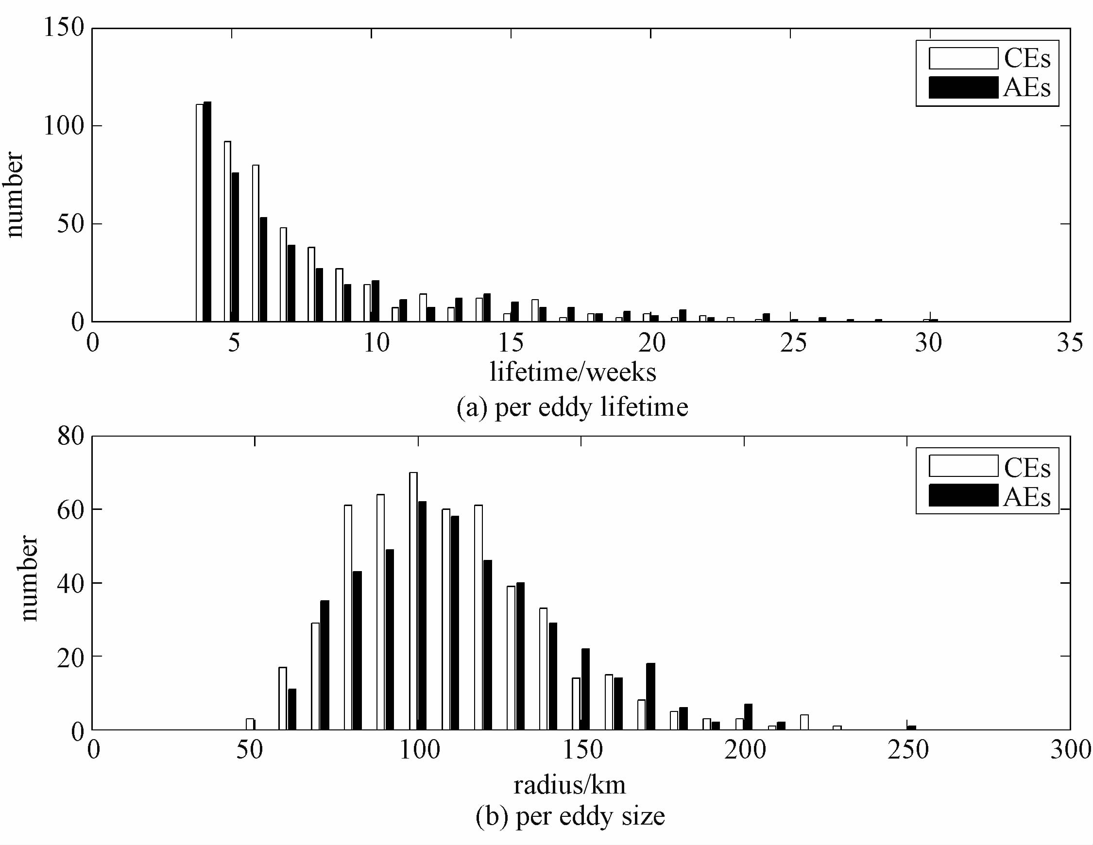
2 Results and discussion 2.1 Eddy number, size and lifetimeApproximately 7 254 eddies were identified in the SCS (depth over 200 m), including 3 632 CEs and 3 622 AEs, which responds to 491 cyclonic tracks and 445 anticyclonic tracks with lifetime ≥4 weeks. Eddy radius ranges from 49.2 km to 257.1 km, with an average value of 111.2 km. Eddy size number distribution deviates from a Gaussian with a distinct skewness towards the larger size and a peak at 100 km for each of eddy polarities (Fig. 1(b)). The mean size is 109.3 km for CEs and 113.3 km for AEs. 82.7% of the eddies have radiuses ranging between 70 km and 150 km, only 15 eddies have radiuses larger than 200 km. For distribution of eddy lifetime (Fig. 1(a)), eddy number decreases in a general manner with lifetime for both eddy polarities. About 81.4% eddies have lifetimes shorter than 10 weeks. There are more AEs than CEs, for lifetime longer than 12 weeks or size lager than 150 km. For shorter lifetime or smaller size it is the opposite.

|
Download:
|
| Fig. 1 Histogram of eddy number | |
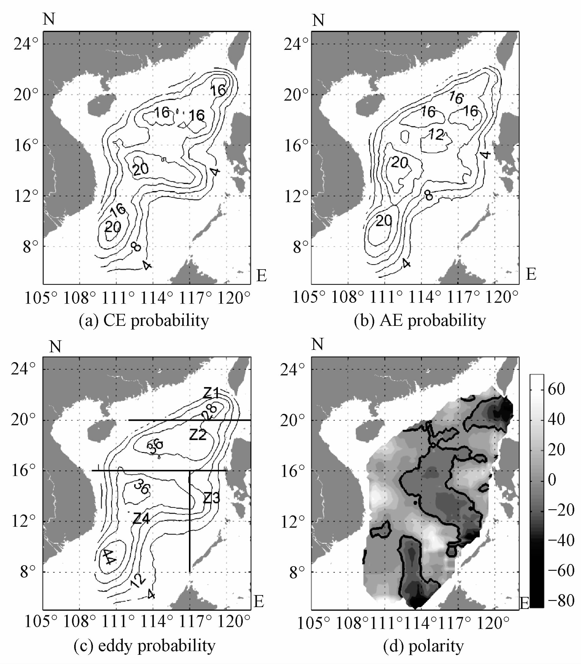
The spatial distribution and birthplace of eddies in the SCS is nonuniform. Figure 2(c) shows the climatological spatial distribution of the eddy probability, which corresponds at each location to the percentage of time that the point flagged by eddies. Regions with high eddy probability tend to be more frequently covered by eddies. The eddy probability has a mean value of 19.3% with the maximal percentage of 44.5%. High probability areas locate in the northeast-southwest direction. Mesoscale activities are commonly observed east of Vietnam, where the eddy probability has two large centers north and south of 12°N respectively, with the probabilities of 30%~44%. In the northeastern region of the SCS, the eddy probability has a level of 25%~37%. High EKE and EAGPE are also observed in these regions(Fig. 6). Although patterns for CEs and AEs are similar (Fig. 2(a) and 2(b)), CEs occurred (~18%) more frequently in the southwest of Taiwan than AEs (~14%). In the northwest of Luzon Island and the southeast of Vietnam AEs dominate. The result was different in that report by Wang et al.[5], in which they concluded that the southwest of Taiwan was dominated by AEs. The discrepancy might be because they focused on eddies with longer lifetime and more CEs were ignored. For eddies with lifetime longer than 18 weeks , 30 AEs and 19 CEs are identified in our study.

|
Download:
|
| Fig. 2 Climatology spatial patterns of eddy occurrence | |
Eddy polarity[19] represents the probability of a point inside a vortex, being inside an AE (positive eddy polarity) or a CE (negative eddy polarity), computed as (PAE-PCE)/(PAE+PCE). Figure 2(d) shows the mean polarity distribution. Three main negative polarity regions can be identified, west of Luzon strait, middle of the SCS and northwest of Brunei with levels of -35% to-5%. These results show a little difference on positions and covered areas, compared with the report of Chen et al.[20]. This might result from the different eddy detection methods and criteria used. Different detection methods can lead to discrepancies in eddies’ centers and sizes. Eddy radius obtained by the winding-angle method is larger than the closed-SSH-contour based method used in this article, which has been confirmed by Yang[21].
2.3 Eddy propagationTo facilitate the discussion, we group eddies into four geographic zones (Fig. 2(c)) according to Wang et al.[5]. The proportions for eddies propagaing with poleward and equatorward deflections due west in Z1 (the southwest of Taiwan) are 29.16%and 43.06% for CEs and 23.94% and 53.53% for AEs, respectively. In Z2 (the northwest of Luzon Island) the proportions are 36.31% and 49.04% for CEs and 41.79% and 44.78% for AEs, respectively.In Z3 (the southwest of Luzon Island) more eddies drift poleward (57.15% for CEs and 55.21% for AEs) than equatorward (33.67% for CEs and 37.5% for AEs). Situation in Z4 (east of Vietnam) is different from the other regions. For CEs the equatorward drift eddies dominate( 50% to 28.05%). While for AEs the situation is opposite(31.94% to 36.11%). The trajectories of eddies in the SCS is rather complicated. A noteworthy feature is that most eddies tend to propagate westward with meridional drift.
On the global sight AEs and CEs have distinct preferences for equatorward and poleward deflections[11]. The opposing meridional deflections of CEs and AEs are expected from the combined effects of the β effect and the self-advection[22]. Eddy-eddy interactions and eddy-mean flow interactions might be the other factors affecting the eddy motion. However, eddies in the SCS do not show these preferences. It seems the propagation of eddies is largely influenced by the circulation in the SCS. Driven by the monsoon system, there is generally a basin-wide cyclonic gyre in winter while during summer a cyclonic gyre north of about 12°N and an anticyclonic gyre south of it[2]. Accordingly eddy propagations have a southwest direction preference in Z1 and Z2, and a northwest direction preference in Z3. The Kuroshio intrusion into the SCS exists all the year round and is stronger in winter than in summer[23]. The Kuroshio flows northwestward into the SCS mainly through the Balintang Channel and flows northeastward out through the Bashi Channel[24]. These may relate to the relatively higher proportions of eastward propagation eddies with meridional drift in Z1. Z4 is another area where eastward propagation eddies with meridional drift frequently occur because of the existence of eastward jet offshore the Vietnam coast.
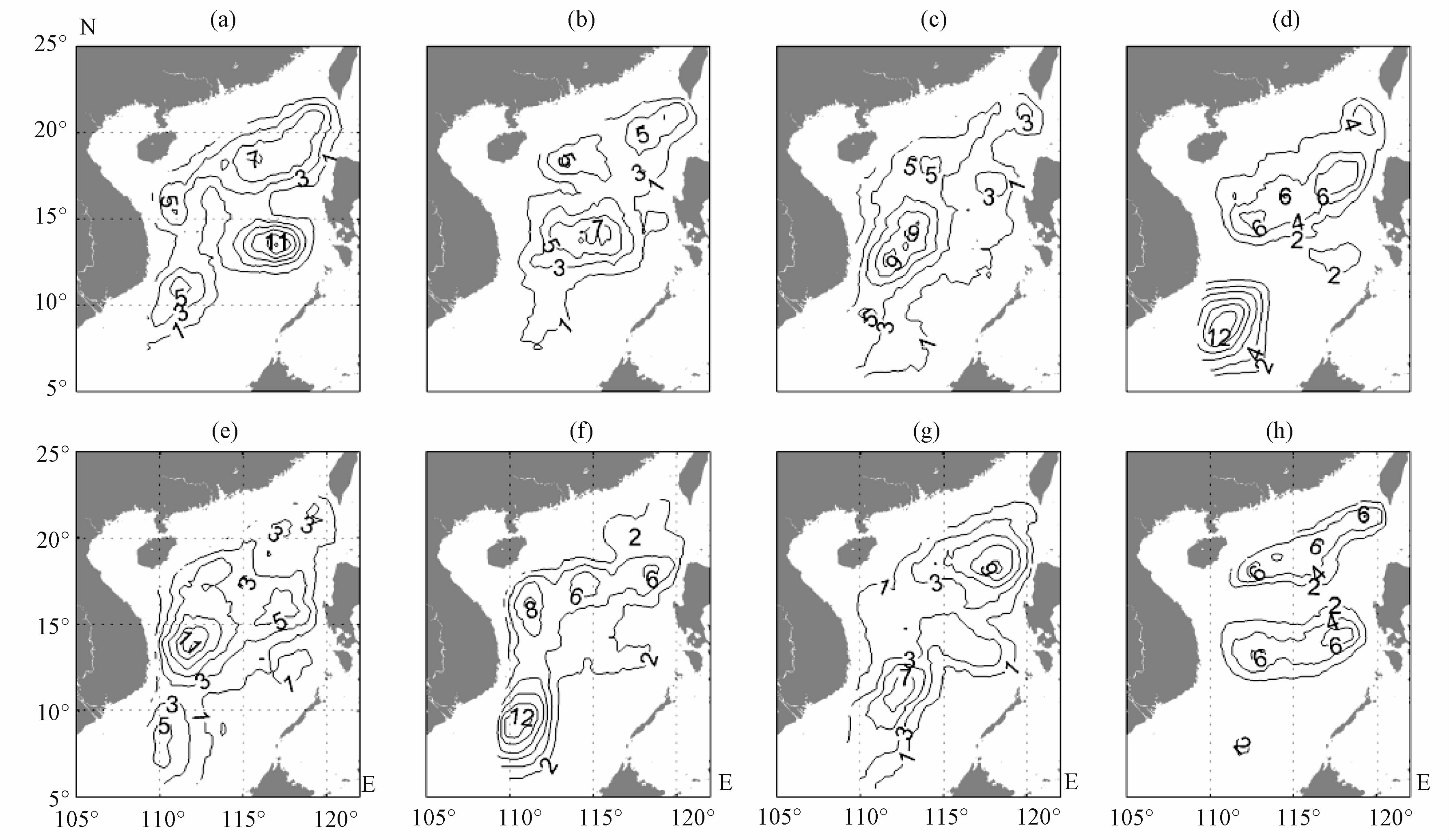
2.4 Seasonal variability of eddyFigure 3 shows the seasonal variations of the spatial distribution of eddy probabilities. Spring and winter seem to be the favorable seasons for the generation of CEs (6.3%) and AEs (6.1%) in Z1. This is also true in Z3, and the proportions are 11.3% for CEs during spring and 7.0% for AEs in winter. Frontal instability at the Kuroshio intrusion could be one mechanism in shedding these AEs in Z1[6]. Cai et al.[25] suggested that the interaction between strong barotropic shelf currents and local topography is a possible reason for the occurrence of AEs in Z3.

|
Download:
|
| Fig. 3 Seasonal variations in climatology spatial patterns of eddy occurrence | |
In Z2 CEs prefer to occur in winter (7.9%) and spring (7.4%), whereas AEs prefer in autumn (9.6%) and summer (8.6%). Metzger and Hurlburt[26] also found AEs tended to form to the west of Babuyan Islands in eastern Z2 in August/September. The intense positive wind stress offshore northwest of Luzon[4] and the (positive) vorticity advected westward from Kuroshio front[27] may attribute to the generation of CEs in winter.
CEs have a high probability center (9.5%) north of 12°N in Z4 during autumn. In winter the high-value center moves southward around (111°E, 9°N) and is enhanced (~13.6%). Then the probability decreased (~6.4%) and the centers move northward in spring. In summer it moves back to the central SCS with the probability increasing up to ~9.5%. While AEs in Z4 prefer to generate north of 12°N in spring (11.7%) and southward intensify in summer (13.8%). In autumn it starts to weaken (8.5%) and moves northeastward, and in winter the probability is the lowest (6.5%) north of 12°N. The southward coastal current off eastern Vietnam encountering the coastal promontory at about 12°N tends to induce the generation of CEs in winter, while in summer the northeastern wind-driven coastal jet separation from the coast of central Vietnam is of benefit to the generation of AEs[28].
2.5 Relationship among eddy, wind, and flowEddy generation mechanisms are nonuniform in different areas of the SCS. Xiu et al.[9] assumed that WSC was a significant factor but not the only factor that accounted for eddy formation. Hwang and Chen[8] compared the WSC and eddies in the central SCS basin. They found that positive (negative) WSC anomaly produced divergence (convergence)in the surface water and the upwelling (downwelling) corresponded to a cold core (warm core) eddy. The wind jets associated with the wintertime intense negative WSC is the main reason for the generation of AEs on southwest of Taiwan in winter[29]. Eddies were generated in the regions to the southeast of Vietnam in winter and off central Vietnam in summer because of wind-driven coastal jet separation and strong flow variability[28]. Chen et al.[20] suggested that eddy number in northern SCS had a good correlation with the strength of background flows. Nan et al.[30] compared ambient geostrophic currents and eddy occurrence patterns on southwest of Taiwan and assumed that the Kuroshio path variation was likely the control factor for eddy generation.
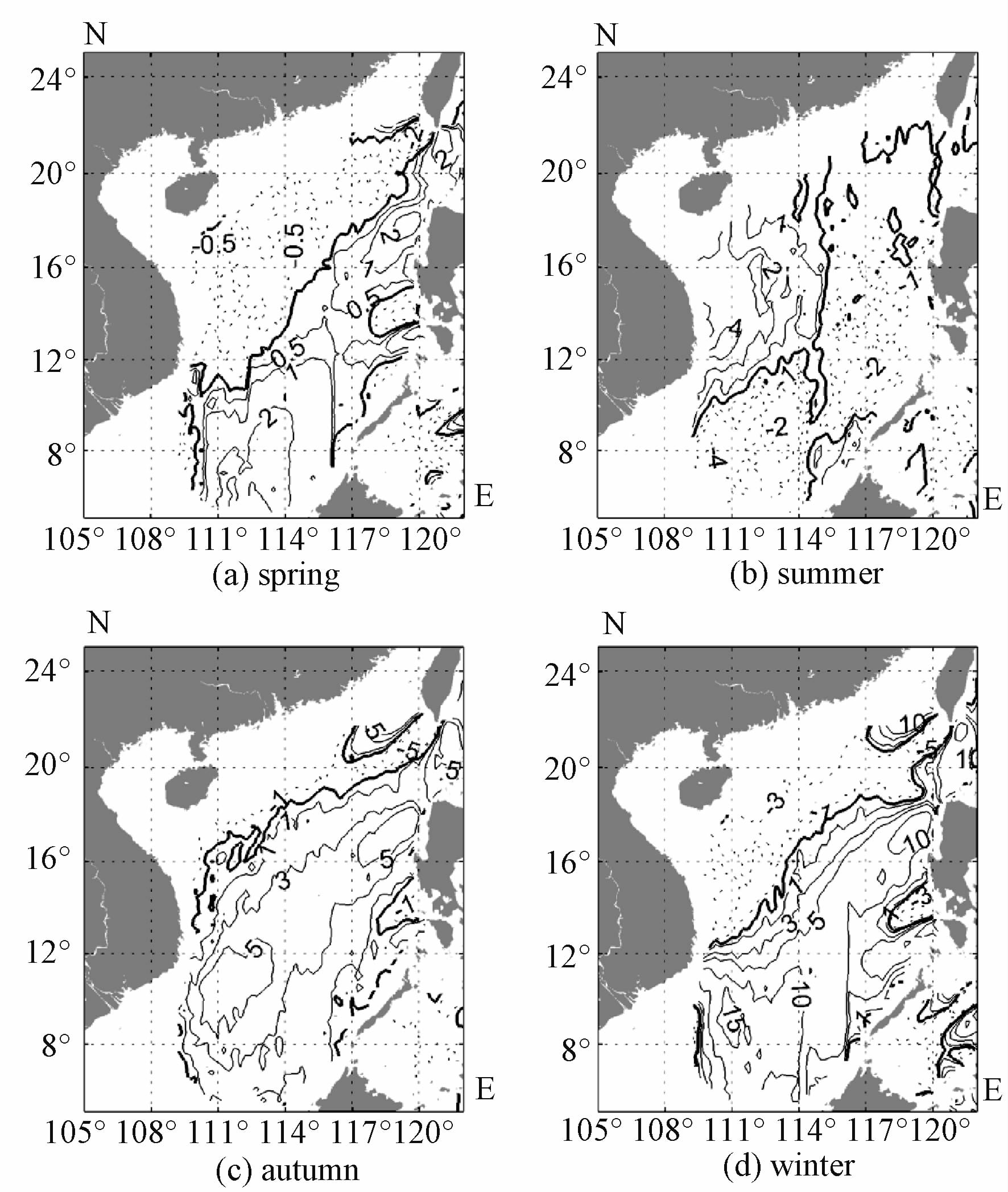
The seasonally reversing monsoon system in the SCS is typically the northeast winds during boreal winter and the southwest winds during boreal summer. Furthermore, the monsoon is stronger in winter and weaker in summer. Figure 4 shows the distribution of seasonal mean WSC in the SCS. The regions with high AE occurrences in Z1 and Z3 (Fig. 3(h)) and the southern side of Z4 (Fig. 3(f)) correspond to strong negative WSC in winter and summer, respectively. The regions with high CE occurrences in Z2 and Z4 (Fig. 3(d)) correspond to strong positive WSC in winter. However, the consistency is not shown elsewhere. The WSC pattern in autumn is similar to that in winter except for being a little weaker.The eddy occurrence pattern in autumn (Fig. 3(c) and (g)) is quite different from that in winter. The north of 12°N in Z4 has the highest AE occurrence in spring (Fig. 3(d)), while there is no corresponding negative WSC. In Z3 there is the highest CE probability during spring but no related positive WSC. These discrepancies between the seasonal WSC patterns and the seasonal eddy probability patterns lead us to conclude that although it may benefit for eddy forming to change the SLA though Ekman pumping, the WSC cannot be the only factor directly controlling the eddy formation in the SCS.

|
Download:
|
| Fig. 4 Seasonal changes in the climatology mean WSC spatial patterns | |
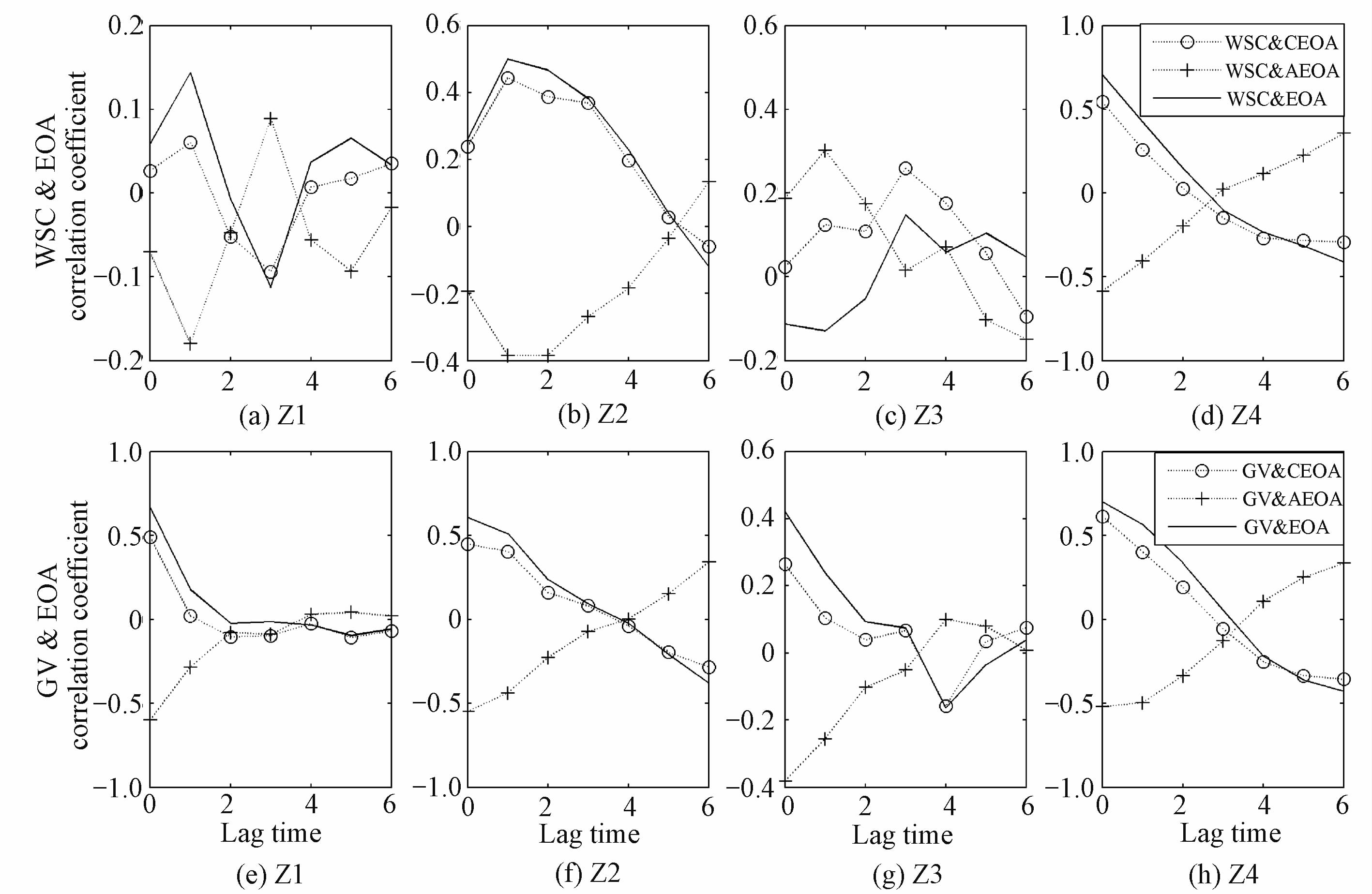
To compare the effect of local WSC on eddy formation, the time series of monthly mean WSC, average geographic vorticity (GV), and eddy-occupied area of each region are estimated. GV is calculated by means of the formula ∂/∂x(-g/f∂(ADT)/∂(y))-∂/∂y(g/f∂(ADT)/∂x). EOA is computed as the difference between cyclonic EOA (CEOA) and anticyclonic EOA (AEOA). A correlation analysis among monthly WSC, GV, andEOA is conducted (Table 1). The correlation coefficients between EOA and GV show positive high-values in all areas, which are 0.67, 0.60, 0.42, and 0.7 (all above 95% significance level) in Z1, Z2, Z3, and Z4, respectively. It is positive (negative) between CEOA (AEOA) and GV. However, the correlation coefficient between WSC and EOA varies considerably in different regions of the SCS. There is remarkable positive correlation(O.F) in Z4 area. It is relatively weak (0.26) in Z2 area, but still above 95% significant level. While the correlation coefficient in Z3 area shows a weak negative correlation(-0.11).That is contributed by the correlation with AEOA, which is ~-0.19. The correlation in Z1 area is rather weak. These results indicate that background flow plays a direct role in eddy formation in the whole SCS, while the immediate role of WSC is different in various regions. In Z4 area, both factors on the direct eddy formation are equally relevant. In other areas GV plays a more relevant role than WSC. Moreover, WSC does not show direct relation on eddy formation in Z1. Lag correlation between WSC and EOA shows that the best relevance appears when EOA is one month lagged behind WSC in all regions except for Z4, in which the correlation deceases as EOA lags behind WSC (Fig. 5). However, the best correlation between GV and EOA occurs when there is no lag at all. This suggests that GV has immediate effect on eddy formation while WSC’s instantaneity only shows in Z4 area.
|
|
Table 1 Correlation coefficient (R) and corresponding significance (P) analysisa |

|
Download:
|
| Fig. 5 Lag correlation coefficients between WSC and EOA and between GV and EOA in each area | |
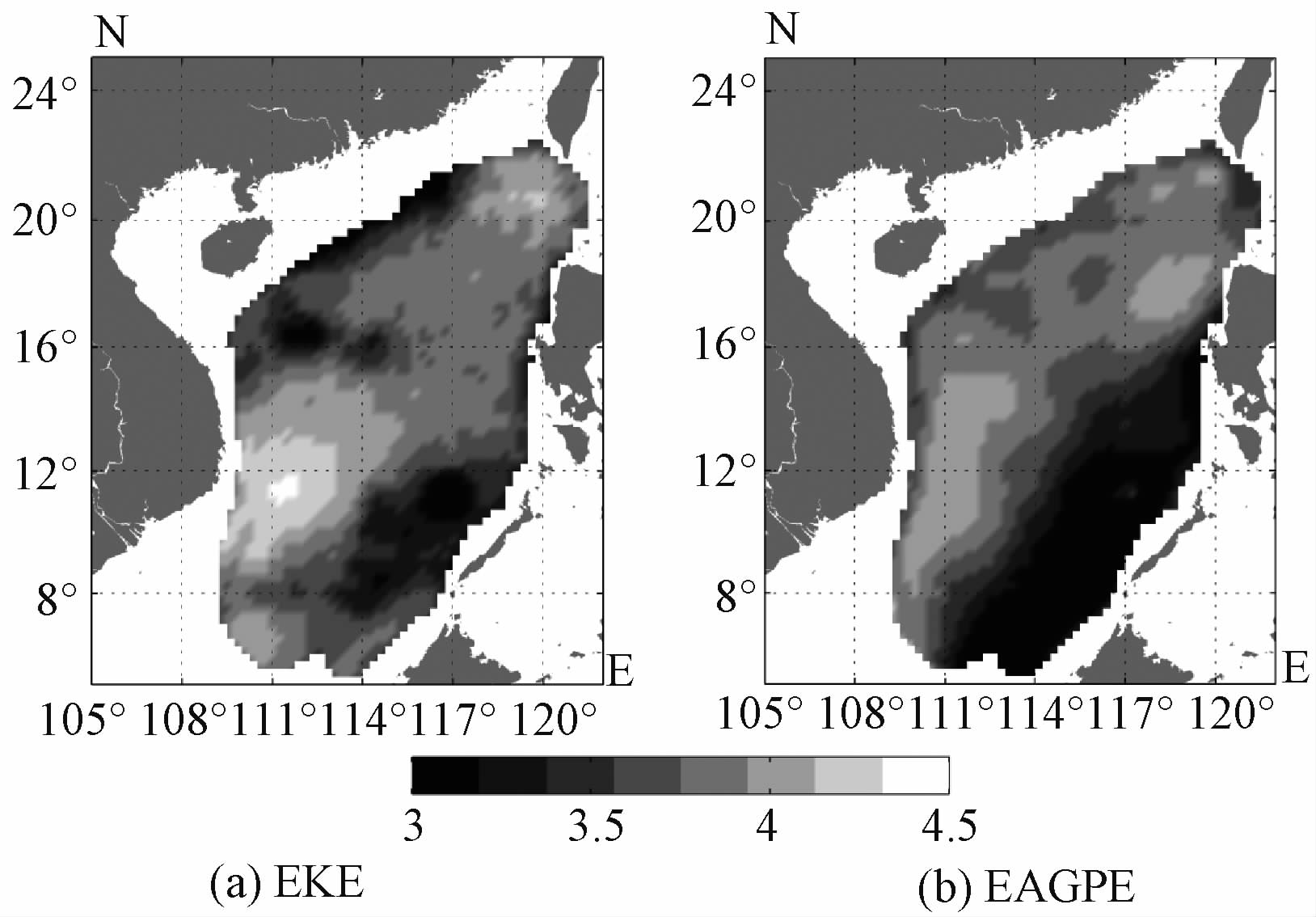
Figure 6 gives the distribution of EKE and EAGPE in the SCS. The total amount of EKE (EAGPE) is estimated at 0.012 2 EJ (0.008 7 EJ). Unlike that in the open ocean, the eddy energy in the inner SCS is confined in the upper layer[31]. The EKE distribution shows two high value centers, one locating to the southwest of Taiwan and the other in the eastern area off the Vietnamese coast. For EAGPE there are three high value centers which contain the former two regions and an additional one to the northwest of Luzon. Both patterns show great consistency with the eddy probability (Fig. 2). To quantify the attribution of wind energy to eddy energy, we follow Wunsch[32]and calculate the rate of wind energy input to the surface currents by the scalar product of wind stress and surface current velocity, w=τ·u>. Most of the wind energy input occurs offshore Vietnam with magnitude of around 0.13 W·m-2 in winter and 0.07 W·m-2 in summer, respectively. Correlation analysis between monthly mean wind power input (WPI) and the monthly mean EKE (EAGPE)in each region is studied (Table 1). Positive correlation exists in most regions of the SCS except Z3. This indicates that wind stress is energy source of eddy in all regions except Z3. Z1 and Z2 have significant positive correlation between EKE and WPI. Good negative correlation between EAGPE and WPI is showed in Z3. Both correlations of the two show equal importance in Z4. However, the correlation coefficients are less than 0.30, indicating that the local WPI has limited effects on the eddy energy. What controls the eddy energy is beyond the scope of this study and needs further research.

|
Download:
|
| Fig. 6 Horizontal distributions of mean EKE (a) and EAGPE (b) in lg form (unit: J·m-2) | |
Using a 19.5 (October 1992 to April 2012) years eddy dataset, we examined eddy activities in the SCS. A total of 3 632 CEs and 3 622 AEs are identified, which responds to 491 cyclonic tracks and 445 anticyclonic tracks. The radius of these eddies ranges from 49.2 km to 257.1 km, with an average value of 111.2 km. Eddy number decreases in a general manner with increasing lifetime for both eddy polarities. About 81.4% of eddies have lifetimes shorter than 10 weeks.
There are three high eddy occurrence areas lying southwest of Taiwan, northwest of Luzon, and offshore Vietnam. These areas correspond to the active eddy energy regions. Most eddies prefer a westward propagation with meridional deflections. Eastward propagating eddies occurred more often in Z1 and Z4 where the Kuroshio intrusion and the east jet offshore Vietnam significantly influence the local circulation .
Eddy occurrence has a notable seasonal pattern in the SCS. CEs (AEs) are in favor of spring (winter) in Z1 and Z3. In Z2 CEs prefer to occur in winter and spring, whereas AEs prefer in autumn and summer. CEs (AEs) in Z4 are generated most likely in winter (summer).
There exists a remarkable positive correlation coefficient between the GV and EOA in the SCS. However, the effects of WSC on EOA are different in different areas of the SCS. It has an equal relevance on the formation of eddies compared to GV in Z4 area. In Z2 and Z3 the correlation coefficients are relatively small. However, the relationship in Z1 shows no direct effect of WSC on eddy formation. We further discuss the wind energy attribution to eddy energy. In Z4 both EKE and EAGPE have significant positive correlations with WPI. In Z1 and Z2 only EKE shows significantly positive correlation with WPI, whereas in Z3 only EAGPE is negatively correlated to WPI. It turns out that WPI has limited effects on eddy energy. Further research needs to be done on the control factors of eddy energy.
| [1] | Wyrtki K. Physical oceanography of the southeast Asian waters, scientific results of marine investigations of the south China Sea and the Gulf of Thailand, NAGA Rep. 2 [R]. Scripps Inst of Oceanogr, La Jolla, California, 1961:195. |
| [2] | Liu Q, Kaneko A, Jilian S. Recent progress in studies of the South China Sea circulation[J]. Journal of oceanography , 2008, 64 (5) :753–762. DOI:10.1007/s10872-008-0063-8 |
| [3] | Jilian S. Overview of the South China Sea circulation and its influence on the coastal physical oceanography outside the Pearl River Estuary[J]. Continental Shelf Research , 2004, 24 (16) :1745–1760. DOI:10.1016/j.csr.2004.06.005 |
| [4] | Qu T. Upper-layer circulation in the South China Sea[J]. Journal of Physical Oceanography , 2000, 30 (6) :1450–1460. DOI:10.1175/1520-0485(2000)030<1450:ULCITS>2.0.CO;2 |
| [5] | Wang G, Su J, Chu P C. Mesoscale eddies in the South China Sea observed with altimeter data[J]. Geophysical Research Letters , 2003, 30 (21) :2121. DOI:10.1029/2003GL018532 |
| [6] | Wang L, Koblinsky C J, Howden S. Mesoscale variability in the South China Sea from the TOPEX/Poseidon altimetry data[J]. Deep Sea Research Part I: Oceanographic Research Papers , 2000, 47 (4) :681–708. DOI:10.1016/S0967-0637(99)00068-0 |
| [7] | Li L, Nowlin W D, Jilian S. Anticyclonic rings from the Kuroshio in the South China Sea[J]. Deep-Sea Research Part I , 1998, 45 (9) :1469–1482. DOI:10.1016/S0967-0637(98)00026-0 |
| [8] | Hwang C, Chen S A. Circulations and eddies over the South China Sea derived from TOPEX/Poseidon altimetry[J]. Journal of Geophysical Research: Oceans (1978-2012) , 2000, 105 (C10) :23943–23965. DOI:10.1029/2000JC900092 |
| [9] | Xiu P, Chai F, Shi L, et al. A census of eddy activities in the South China Sea during 1993-2007[J]. Journal of Geophysical Research: Oceans (1978-2012) , 2010, 115 :C03012. DOI:10.1029/2009JC005657 |
| [10] | Yuan D, Han W, Hu D. Anticyclonic eddies northwest of Luzon in summer-fall observed by satellite altimeters[J]. Geophysical research letters , 2007, 34 (13) :L13610. DOI:10.1029/2007GL029401 |
| [11] | Chelton D B, Schlax M G, Samelson R M. Global observations of nonlinear mesoscale eddies[J]. Progress in Oceanography , 2011, 91 (2) :167–216. DOI:10.1016/j.pocean.2011.01.002 |
| [12] | Yuan D, Han W, Hu D. Surface Kuroshio path in the Luzon Strait area derived from satellite remote sensing data[J]. Journal of Geophysical Research: Oceans (1978-2012) , 2006, 111 (C11) :C11007. DOI:10.1029/2005JC003412 |
| [13] | Xu C, Shang X D, Huang RX. Horizontal eddy energy flux in the world oceans diagnosed from altimetry data[J]. Scientific Rreports , 2014, 4 :5316. DOI:10.1038/srep05316 |
| [14] | Wu J. Wind-stress coefficients over sea surface from breeze to hurricane[J]. Journal of Geophysical Research: Oceans (1978-2012) , 1982, 87 (C12) :9704–9706. DOI:10.1029/JC087iC12p09704 |
| [15] | Huang R X. Ocean circulation: wind-driven and thermohaline processes[M]. Cambridge: Cambridge University Press, 2010 : 806 . |
| [16] | Ferrari R, Wunsch C. The distribution of eddy kinetic and potential energies in the global ocean[J]. Tellus A , 2010, 62 (2) :92–108. DOI:10.3402/tellusa.v62i2.15680 |
| [17] | Xu C, Shang X D, Huang R X. Estimate of eddy energy generation/dissipation rate in the world ocean from altimetry data[J]. Ocean Dynamics , 2011, 61 (4) :525–541. DOI:10.1007/s10236-011-0377-8 |
| [18] | Flierl G R. Models of vertical structure and the calibration of two-layer models[J]. Dynamics of Atmospheres and Oceans , 1978, 2 (4) :341–381. DOI:10.1016/0377-0265(78)90002-7 |
| [19] | Chaigneau A, Eldin G, Dewitte B. Eddy activity in the four major upwelling systems from satellite altimetry (1992-2007)[J]. Progress in Oceanography , 2009, 83 (1) :117–123. |
| [20] | Chen G, Hou Y, Chu X. Mesoscale eddies in the South China Sea: mean properties, spatiotemporal variability, and impact on thermohaline structure[J]. Journal of Geophysical Research: Oceans (1978-2012) , 2011, 116 (C6) :C06018. DOI:10.1029/2010JC006716 |
| [21] | Yang G. A study on the mesoscale eddies in the Northwestern Pacific Ocean [D]. Qingdao: Institute of Oceanology, Chinese Academy of Sciences, 2013(in Chinese). |
| [22] | Cushman-Roisin B. Introduction to Geophysical Fluid Dynamics[M]. Prentice-Hall: Englewood Cliffs, NJ, 1994 . |
| [23] | Shaw P T. The seasonal variation of the intrusion of the Philippine Sea water into the South China Sea[J]. Journal of Geophysical Research: Oceans (1978-2012) , 1991, 96 (C1) :821–827. DOI:10.1029/90JC02367 |
| [24] | Liang W D, Yang Y J, Tang T Y, et al. Kuroshio in the Luzon Strait[J]. Journal of Geophysical Research: Oceans (1978-2012) , 2008, 113 (C8) :C08048. DOI:10.1029/2007JC004609 |
| [25] | Cai S, Su J, Gan Z, et al. The numerical study of the South China Sea upper circulation characteristics and its dynamic mechanism, in winter[J]. Continental Shelf Research , 2002, 22 (15) :2247–2264. DOI:10.1016/S0278-4343(02)00073-0 |
| [26] | Metzger E J, Hurlburt H E. The nondeterministic nature of Kuroshio penetration and Eddy shedding in the South China Sea[J]. Journal of Physical Oceanography , 2001, 31 (7) :1712–1732. DOI:10.1175/1520-0485(2001)031<1712:TNNOKP>2.0.CO;2 |
| [27] | Liu X, Su J. A reduced gravity model of the circulation in the South China Sea[J]. Oceanologia et Limnologia Sinica , 1991, 23 (2) :167–174. |
| [28] | Gan J, Qu T. Coastal jet separation and associated flow variability in the southwest South China Sea[J]. Deep Sea Research Part I: Oceanographic Research Papers , 2008, 55 (1) :1–19. DOI:10.1016/j.dsr.2007.09.008 |
| [29] | Wang G, Chen D, Su J. Winter eddy genesis in the eastern South China Sea due to orographic wind jets[J]. Journal of Physical Oceanography , 2008, 38 (3) :726–732. DOI:10.1175/2007JPO3868.1 |
| [30] | Nan F, Xue HJ, Xiu P, et al. Oceanic eddy formation and propagation southwest of Taiwan[J]. J Geophys Res-Oceans , 2011, 116, C12045 . DOI:10.1029/2011JC007386 |
| [31] | Yang H, Wu L, Liu H, et al. Eddy energy sources and sinks in the South China Sea[J]. Journal of Geophysical Research: Oceans , 2013, 118 (9) :4716–4726. DOI:10.1002/jgrc.20343 |
| [32] | Wunsch C. The work done by the wind on the oceanic general circulation[J]. Journal of Physical Oceanography , 1998, 28 (11) :2332–2340. DOI:10.1175/1520-0485(1998)028<2332:TWDBTW>2.0.CO;2 |