Stochastic Poisson systems are defined as the form^[1]

$\left\{\begin{array}{l}\mathrm{d} \boldsymbol{y}(t)=\boldsymbol{B}(\boldsymbol{y}(t))\left(\nabla H_0(\boldsymbol{y}(t)) \mathrm{d} t+\right. \\ \left.\sum\limits_{r=1}^s \nabla H_r(\boldsymbol{y}(t)) \circ \mathrm{d} W_r(t)\right), \\ \boldsymbol{y}\left(t_0\right)=\boldsymbol{y}_0, \end{array}\right.$

(1)

where y(t)=(y₁, …, y_n)^T, B(y)=(b_ij(y))_n×n is a skew-symmetric matrix, and satisfies the condition

$\begin{gathered}\sum\nolimits_{v=1}^n\left(\frac{\partial b_{i j}(\boldsymbol{y})}{\partial y_v} b_{v k}(\boldsymbol{y})+\frac{\partial b_{j k}(\boldsymbol{y})}{\partial y_v} b_{v i}(\boldsymbol{y})+\right. \\ \left.\frac{\partial b_{k i}(\boldsymbol{y})}{\partial y_v} b_{v j}(\boldsymbol{y})\right)=0, \end{gathered}$

(2)

for all i, j, k∈{1, …, n}.H_r(y), r=0, …, s are smooth scalar functions. W(t)=(W₁(t), …, W_s(t)) is an s-dimensional standard Wiener process, and ○ stands for the Stratonovich product. We assume that B(y) is of constant rank 2m=n-l, 0≤l<n.

A skew-symmetric matrix B(y) with property (2) can define the Poisson bracket {F, G}(y) of two smooth functions F(y) and G(y) as Refs. [1-2]

$\{F, G\}(\boldsymbol{y}):=\sum\nolimits_{i, j=1}^n \frac{\partial F(\boldsymbol{y})}{\partial y_i} b_{i j}(\boldsymbol{y}) \frac{\partial G(\boldsymbol{y})}{\partial y_j}, $

or equivalently in the form

$\{\boldsymbol{F}, G\}(\boldsymbol{y}):=\nabla F(\boldsymbol{y}){ }^{\mathrm{T}} \boldsymbol{B}(\boldsymbol{y}) \nabla G(\boldsymbol{y}).$

It is known that almost surely the phase flow φ_{t, ω}: y₀→y(t) of the stochastic Poisson system (1) preserves the Poisson structure^[1],

$\frac{\partial \boldsymbol{y}(t)}{\partial \boldsymbol{y}_0} \boldsymbol{B}\left(\boldsymbol{y}_0\right) \frac{\partial \boldsymbol{y}(t)^{\mathrm{T}}}{\partial \boldsymbol{y}_0}=\boldsymbol{B}(\boldsymbol{y}(t)), \forall t \geqslant t_0.$

(3)

A function C(y) is called Casimir function of the system (1) if

$\nabla C(\boldsymbol{y})^{\mathrm{T}} \boldsymbol{B}(\boldsymbol{y})=0, \quad {\rm for\; all} \;\boldsymbol{y}.$

It is not difficult to prove that each Casimir function C(y) is an invariant for the system (1)^[1].

If n=2m and $\boldsymbol{B}(\boldsymbol{y})=\left(\begin{array}{ll}\mathit{\pmb{0}} & -\boldsymbol{I}_m \\ \boldsymbol{I}_m & \mathit{\pmb{0}}\end{array}\right)$, where I_m denotes an m-dimensional identity matrix, the stochastic Poisson system (1) degenerates to the stochastic canonical Hamiltonian system. The phase flow of a stochastic Hamilton system preserves the symplectic structure^[3-4]. The Poisson structure of stochastic Poisson systems is an extension of the symplectic structure. For stochastic Poisson systems, there arised some numerical results in recent years. For a special class of stochastic Poisson systems, numerical methods are proposed in Ref. [5] and Ref. [6] respectively, where the method proposed in Ref. [5] can exactly preserve quadratic Casimir functions and the energy, while the method given in Ref. [6] is energy-preserving with the ability of arriving any prescribed order. In Ref. [7], for stochastic Poisson systems of even dimensions, the structure-preserving Runge-Kutta and partitioned Runge-Kutta methods are proposed. The Darboux-Lie theorem and symplectic methods are used to obtain structure-preserving numerical schemes for stochastic Poisson systems in Ref. [1].

In this paper, we consider the following stochastic Lotka-Volterra (L-V) system with Stratonovich white noise^{[5, 8]}

$\left\{\begin{array}{l}\mathrm{d} \boldsymbol{y}(t)=\boldsymbol{B}(\boldsymbol{y}(t)) \nabla H(\boldsymbol{y}(t))(\mathrm{d} t+c \circ \mathrm{d} W(t)), \\ \boldsymbol{y}\left(t_0\right)=\boldsymbol{y}_0, \end{array}\right.$

(4)

with

$\begin{aligned} & H(\boldsymbol{y})=\sum\nolimits_{i=1}^n \beta_i y_i-p_i \ln y_i, \\ & \boldsymbol{B}(\boldsymbol{y})=\operatorname{diag}\left(y_1, \cdots, y_n\right) \boldsymbol{B} \operatorname{diag}\left(y_1, \cdots, y_n\right), \end{aligned}$

(5)

where β_i≠0(i=1, …, n), B is a skew-symmetric constant matrix and c>0 measures the size of the perturbation. Moreover we assume the Assumption 2.1 holds. It was proved in Ref. [8] that, under Assumption 2.1, for any given y₀>0, the system (4)-(5) has a unique solution which is positive for all t≥t₀ almost surely. Hereby and in the sequel we write a vector a>0 to mean that each element of a is positive. Meanwhile, the system (4)-(5) is a stochastic Poisson system, with Casimir functions C(y)=α₁lny₁+…+α_nlny_n, α=(α₁, …, α_n)^T∈Ker B and Hamiltonian H(y) which is smooth for y>0.

In this paper, we transform the stochastic L-V system to a stochastic Hamiltonian system by coordinate transformation. Then we apply the midpoint method, which is a symplectic scheme, to the stochastic Hamiltonian system and by using the inverse transformation to obtain the numerical scheme for the stochastic L-V system. This method is shown to preserve the Poisson structure and Casimir functions of the stochastic L-V system. We further prove that the method is of root mean-square convergence order 1.

1 A Poisson integrator 1.1 The Darboux-Lie theorem

The Darboux-Lie theorem is as follows.

Theorem 1.1    (see Ref. [2]) Suppose that the matrix B(y) defines a Poisson bracket and is of constant rank n-l=2m in a neighborhood of $\boldsymbol{y}_0 \in \mathbb{R}^n$. Then there exist functions P₁(y), …, P_m(y), Q₁(y), …, Q_m(y), and C₁(y), …, C_l(y) satisfying

$\begin{array}{lll}\left\{P_i, P_j\right\}=0, & \left\{P_i, Q_j\right\}=-\delta_{i j}, & \left\{P_i, C_v\right\}=0, \\ \left\{Q_i, P_j\right\}=\delta_{i j}, & \left\{Q_i, Q_j\right\}=0, & \left\{Q_i, C_v\right\}=0, \\ \left\{C_k, P_j\right\}=0, & \left\{C_k, Q_j\right\}=0, & \left\{C_k, C_v\right\}=0, \end{array}$

(6)

for i, j∈{1, …, m}, v∈{1, …, l} on a neighborhood of y₀. The gradients of P_i, Q_j, C_v, (i, j∈{1, …, m}, v∈{1, …, l}) are linearly independent, so that the $\mathbb{R}^n \longrightarrow \mathbb{R}^n$ mapping θ(y): y→(P₁(y), …, P_m(y), Q₁(y), …, Q_m(y), C₁(y), …, C_l(y)) constitutes a local change of coordinates to canonical form.

If we denote y-=(Z(y)^T, C(y)^T)^T, where

$\begin{gathered}\boldsymbol{Z}(\boldsymbol{y})=\left(\boldsymbol{P}(\boldsymbol{y})^{\mathrm{T}}, \boldsymbol{Q}(\boldsymbol{y})^{\mathrm{T}}\right)^{\mathrm{T}}, \\ \boldsymbol{P}(\boldsymbol{y})=\left(P_1(\boldsymbol{y}), \cdots, P_m(\boldsymbol{y})\right)^{\mathrm{T}}, \\ \boldsymbol{Q}(\boldsymbol{y})=\left(Q_1(\boldsymbol{y}), \cdots, Q_m(\boldsymbol{y})\right)^{\mathrm{T}}, \\ \boldsymbol{C}(\boldsymbol{y})=\left(C_1(\boldsymbol{y}), \cdots, C_l(\boldsymbol{y})\right)^{\mathrm{T}}, \end{gathered}$

by the Darboux-Lie theorem, the system (4) can be transformed to ^[1]

$\left\{\begin{array}{l}\mathrm{d} \boldsymbol{Z}=\boldsymbol{J}^{-1} \nabla_Z K(\boldsymbol{Z}, \boldsymbol{C})(\mathrm{d} t+c \circ \mathrm{d} W(t)), \\ \mathrm{d} \boldsymbol{C}=0, \end{array}\right.$

(7)

which is a stochastic Hamiltonian system (SHS) with constant parameter vector C, and K(Z, C)=K(y)=H(y), $\boldsymbol{J}^{-1}=\left(\begin{array}{ll}\mathit{\pmb{0}} & -\boldsymbol{I}_m \\ \boldsymbol{I}_m & \mathit{\pmb{0}}\end{array}\right)$. K is smooth owing to the smoothness of H.

According to the results in Ref. [1], applying a symplectic scheme to SHS (7) and then transforming the scheme back to system (4) by the inverse transformation y=θ^-1(y), one gets a stochastic Poisson integrator for the stochastic Poisson system (4), which can preserve both the Poisson structure and the Casimir functions of system (4) almost surely.

1.2 The numerical scheme

As mentioned above, stochastic Poisson integrators can be obtained by using symplectic methods to the SHS arising from the coordinate transformation. It is well-known that the midpoint method is a symplectic method for SHS^[9]. Therefore we propose a numerical scheme for system (4) derived from the transformation of the midpoint scheme, which we call the transformed midpoint (TM) method in the sequel.

The TM method:

(a) By the Darboux-Lie theorem, we find a coordinate transformation θ(y): y→y=(Z(y)^T, C^T)^T, which transforms system (4) with initial value y₀ to SHS (7) with initial value Z₀=(P(y₀)^T, Q(y₀)^T)^T.

(b) Apply the midpoint method to SHS (5)

$\boldsymbol{Z}_{j+1}=\boldsymbol{Z}_j+\boldsymbol{J}^{-1} \nabla_z K\left(\frac{\boldsymbol{Z}_{j+1}+\boldsymbol{Z}_j}{2}, \boldsymbol{C}\right)\left(h+c \Delta \hat{W}_j\right), $

(8)

where h is the time step and $\Delta \hat{W}_j(j=0, 1, \cdots)$ are truncated Wiener increments (explained below).

(c) Solve equation (6) for Z_j+1, then use the inverse transformation y_j+1=θ^-1(y_j+1) with y_j+1=(Z_j+1^T, C^T)^T to get the numerical solution y_j+1(j=0, 1, …) for system (4).

In equation (8), $\Delta \hat{W}_j: =\sqrt{h} \zeta_j$ is a truncation of $\Delta W_j=\sqrt{h} \xi_j$, where $\xi_j \sim \mathcal{N}(0,1)$ and

$\zeta_j=\left\{\begin{array}{l}\xi_j, \text { if }\left|\xi_j\right| \leqslant A_h, \\ A_h, \text { if } \xi_j>A_h, \\ -A_h, \text { if } \xi_j<-A_h, \end{array}\right.$

where $A_h: =\sqrt{2 k|\ln (h)|}$ (for an integer k≥1)^[9]. Moreover, one has the following estimates^[9-10]:

$\mathbb{E}\left[\xi_j-\zeta_j\right]^2 \leqslant h^2 , $

(9)

$\begin{gathered}0 \leqslant \mathbb{E}\left[\xi_j^2-\zeta_j^2\right]=(1+2 \sqrt{2 k|\ln (h)|}) h^k, \\ \mathbb{E}\left[\xi_j^2-\zeta_j^2\right]^2 \leqslant 27 h .\end{gathered}$

As discussed in Ref. [9], such a truncation is a remedy to fix the issue in implementing an implicit scheme caused by the unboundedness of ΔW_j (j=0, 1, …). By choosing sufficiently large parameter k, the truncation error can be merged into the error of the numerical scheme, and for a method of root mean-square order l, it is sufficient to choose k≥2l. Here in this paper we take k=4 in A_h which is sufficient for our discussion.

Remark 1.1    With the truncation of ΔW_j, the fixed point iteration by solving equation (8) for Z_j+1 can converge for sufficiently small h, similar to the discussion in Refs.[9, 11].

Remark 1.2    The Darboux-Lie transformation θ(y) varies for different concrete problems, usually found by solving the equations in (6).

Then by the discussion in section 1.1 we have the following conclusion.

Theorem 1.2    The TM method preserves the Poisson structure and Casimir functions of the Stochastic L-V System (4)-(5).

2 Convergence order

In this section we will prove the root mean-square convergence order of the TM method.

Assumption 2.1    (see Ref. [8]) Assume that for the parameters β=(β₁, …, β_n)^T, p=(p₁, …, p_n)^T of the system (4)-(5), there exists a real number $s_0 \in \mathbb{R}$ and a vector α∈KerB such that

$\left\{\begin{array}{l}s_0 \boldsymbol{\beta}>0 ,\\ -s_0 \boldsymbol{p}+\boldsymbol{\alpha}<0 .\end{array}\right.$

(10)

Lemma 2.1    (see Ref. [8]) Under Assumption 2.1, for any given initial value y₀>0, the exact solution of system (4)-(5) is almost surely bounded.

Based on Lemma 2.1, we can prove the boundedness of the numerical solution of the TM method. We assume the numerical approximation is performed on the time interval t∈[t₀, T], and t_N=T.

Theorem 2.1    Under Assumption 2.1, given y₀>0, the numerical solution {y_j}(j=1, …, N) arising from the TM method is bounded almost surely.

Proof    Given y₀>0, by Lemma 2.1, the exact solution y(t) of system (4)-(5) is almost surely bounded. Since θ(y) is continuous by the Darboux-Lie theorem (θ′(y) exists and invertible), the solution of system (7) is almost surely bounded. This means there are constants L₁, L₂ such that (P(y)^T, Q(y)^T)^T∈[L₁, L₂]^2m almost surely. For a vector $\boldsymbol{a} \in \mathbb{R}^{2 m}$, we say $\boldsymbol{a} \in\left[L_1, L_2\right]^{2 m}$ to mean that each element of a is in [L₁, L₂].

For Z₀∈[L₁, L₂]^2m, we define

$\boldsymbol{\phi}(\boldsymbol{Z})=\boldsymbol{Z}_0+\boldsymbol{J}^{-1} \nabla_z K\left(\frac{\boldsymbol{Z}+\boldsymbol{Z}_0}{2}, \boldsymbol{C}\right)\left(h+c \Delta \hat{W}_0\right).$

(11)

Then the scheme (6) can be written as

$\boldsymbol{Z}_1=\boldsymbol{\phi}\left(\boldsymbol{Z}_1\right), $

(12)

when j=0. We can use the fixed-point iteration method to solve (12). Select the initial value z of iteration that satisfies 0<‖z-Z₀‖<1, thus z∈[L₁-1, L₂+1]^2m\Z₀. We have

$\begin{aligned}\left\|\boldsymbol{\phi}(\boldsymbol{z})-\boldsymbol{Z}_0\right\| & =\left\|\boldsymbol{J}^{-1} \nabla K\left(\frac{\boldsymbol{z}+\boldsymbol{Z}_0}{2}, \boldsymbol{C}\right)\left(h+c \zeta_0 \sqrt{h}\right)\right\| \\ & =\left\|\boldsymbol{J}^{-1} \nabla K\left(\frac{\boldsymbol{z}+Z_0}{2}, \boldsymbol{C}\right)\right\|\left(h+c\left|\zeta_0\right| \sqrt{h}\right)\end{aligned}$

Since $\frac{\boldsymbol{z}+\boldsymbol{Z}_0}{2} \in\left[L_1-1, L_2+1\right]^{2 m}$, and the function $\boldsymbol{J}^{-1} \nabla K(\boldsymbol{z}, \boldsymbol{C})$ is continuous, we have

$\left\|\boldsymbol{\phi}(\boldsymbol{z})-\boldsymbol{Z}_0\right\| \leqslant K_3\left(h+c\left|\zeta_0\right| \sqrt{h}\right), $

for certain K₃>0. Since $\left|\zeta_0\right| \leqslant A_h=\sqrt{2 k|\ln h|}$, and h|lnh|→0 as h→0, we can choose sufficiently small h₁ such that for h<h₁, $K_3\left(h+c\left|\zeta_0\right| \sqrt{h}\right)$<1, which implies ϕ(z)∈[L₁-1, L₂+1]^2m.

On the other hand, denote

$\boldsymbol{f}(\boldsymbol{z}):=\boldsymbol{J}^{-1} \nabla_z K(\boldsymbol{z}, \boldsymbol{C}), \boldsymbol{g}(\boldsymbol{z}):=c \boldsymbol{J}^{-1} \nabla_z K(\boldsymbol{z}, \boldsymbol{C}), $

then for any z₁, z₂∈[L₁-1, L₂+1]^2m, due to smoothness of K and $\frac{\boldsymbol{z}_i+\boldsymbol{Z}_0}{2} \in\left[L_1-1, L_2+1\right]^{2 m} (i=1, 2)$, it is not difficult to see from (11) that there exists constant K₄>0 such that

$\left\|f\left(\boldsymbol{z}_1\right)-f\left(\boldsymbol{z}_2\right)\right\| \leqslant K_4\left\|\boldsymbol{z}_1-\boldsymbol{z}_2\right\|.$

Choose h₂>0 such that for h<h₂, $K_4 (h+c\left|\zeta_0\right|(\sqrt{h})<1$, which implies $\left\|\boldsymbol{\phi}\left(\boldsymbol{z}_1\right)-\boldsymbol{\phi}\left(\boldsymbol{z}_2\right)\right\|< \left\|\boldsymbol{z}_1-\boldsymbol{z}_2\right\|$. Then for h<h₀: =min{h₁, h₂}, ϕ: [L₁-1, L₂+1]^2m→[L₁-1, L₂+1]^2m is a contraction mapping. According to the contraction mapping principle, the sequence of iterations converges and Z₁∈[L₁-1, L₂+1]^2m.

Expanding the midpoint scheme, by the smoothness of K and the boundedness of Z₀ and Z₁, we get

$\begin{aligned} &\boldsymbol{Z}_1=\boldsymbol{Z}_0+h \boldsymbol{f}\left(\frac{\boldsymbol{Z}_1+\boldsymbol{Z}_0}{2}\right)+g\left(\frac{\boldsymbol{Z}_1+\boldsymbol{Z}_0}{2}\right) \zeta_0 \sqrt{h} \\= & \boldsymbol{Z}_0+\left(\boldsymbol{f}\left(\boldsymbol{Z}_0\right)+\frac{1}{2} \frac{\partial \boldsymbol{f}}{\partial \boldsymbol{z}}\left(\boldsymbol{Z}_0\right)\left(\boldsymbol{Z}_1-\boldsymbol{Z}_0\right)+O(h)\right) h+ \\ & \left(\boldsymbol{g}\left(Z_0\right)+\frac{1}{2} \frac{\partial \boldsymbol{g}}{\partial \boldsymbol{z}}\right)\left(\boldsymbol{Z}_0\right)\left(\boldsymbol{Z}_1-\boldsymbol{Z}_0\right)+ \\ & \left.\frac{1}{8} \frac{\partial^2 \boldsymbol{g}}{\partial \boldsymbol{z}^2}\left(\boldsymbol{Z}_0\right)\left(\boldsymbol{Z}_1-\boldsymbol{Z}_0\right)^2+O(h \sqrt{h})\right) \zeta_0 \sqrt{h} .\end{aligned}$

Then using the relationship (8), we have

$\begin{aligned} \boldsymbol{Z}_{1}= & \boldsymbol{Z}_{0}+\boldsymbol{f}\left(\boldsymbol{Z}_{0}\right) h+\boldsymbol{g}\left(\boldsymbol{Z}_{0}\right) \zeta_{0} \sqrt{h}+ \\ & \frac{1}{2} \frac{\partial \boldsymbol{f}}{\partial z}\left(\boldsymbol{Z}_{0}\right)\left(\boldsymbol{g}\left(\frac{\boldsymbol{Z}_{1}+\boldsymbol{Z}_{0}}{2}\right) \zeta_{0} \sqrt{h}+\boldsymbol{f}\left(\frac{\boldsymbol{Z}_{1}+\boldsymbol{Z}_{0}}{2}\right) h\right) h+ \\ & \left.\frac{1}{2} \frac{\partial \boldsymbol{g}}{\partial z}\left(\boldsymbol{Z}_{0}\right)\left(\boldsymbol{g}\left(\frac{\boldsymbol{Z}_{1}+\boldsymbol{Z}_{0}}{2}\right) \zeta_{0} \sqrt{h}\right)+f\left(\frac{\boldsymbol{Z}_{1}+\boldsymbol{Z}_{0}}{2}\right) h\right) \zeta_{0} \sqrt{h}+ \\ & \frac{1}{8} \frac{\partial^{2} \boldsymbol{g}}{\partial z^{2}}\left(\boldsymbol{Z}_{0}\right)\left(g\left(\frac{\boldsymbol{Z}_{1}+\boldsymbol{Z}_{0}}{2}\right) \zeta_{0} \sqrt{h}+f\left(\frac{\boldsymbol{Z}_{1}+\boldsymbol{Z}_{0}}{2}\right) h\right)^{2} \zeta_{0} \sqrt{h}+ \\ & O\left(h^{2}\right) \\ = & \boldsymbol{Z}_{0}+\boldsymbol{f}\left(\boldsymbol{Z}_{0}\right) h+\boldsymbol{g}\left(\boldsymbol{Z}_{0}\right) \zeta_{0} \sqrt{h}+ \\ & \frac{1}{2} \frac{\partial \boldsymbol{g}}{\partial z}\left(\boldsymbol{Z}_{0}\right) \boldsymbol{g}\left(\boldsymbol{Z}_{0}\right) \zeta_{0}^{2} h+ \\ & \frac{1}{4}\left(\frac{\partial \boldsymbol{g}}{\partial z}\left(\boldsymbol{Z}_{0}\right)\right)^{2} \boldsymbol{g}\left(\boldsymbol{Z}_{0}\right) \zeta_{0}^{3} h \sqrt{h}+ \\ & \frac{1}{2} \frac{\partial \boldsymbol{f}}{\partial z}\left(\boldsymbol{Z}_{0}\right) \boldsymbol{g}\left(\boldsymbol{Z}_{0}\right) \zeta_{0} h \sqrt{h}+\frac{1}{2} \frac{\partial \boldsymbol{g}}{\partial z}\left(\boldsymbol{Z}_{0}\right) \boldsymbol{f}\left(\boldsymbol{Z}_{0}\right) \zeta_{0} h \sqrt{h}+ \\ & \frac{1}{8} \frac{\partial^{2} \boldsymbol{g}}{\partial z^{2}}\left(\boldsymbol{Z}_{0}\right) \boldsymbol{g}^{2}\left(\boldsymbol{Z}_{0}\right) \zeta_{0}^{3} h \sqrt{h}+O\left(h^{2}\right). \end{aligned}$

Since

$ \boldsymbol{Z}\left(t_{1}\right)=\boldsymbol{Z}_{0}+\int_{t_{0}}^{t_{1}} \boldsymbol{f}(\boldsymbol{Z}(s)) \mathrm{d} s+\int_{t_{0}}^{t_{1}} \boldsymbol{g}(\boldsymbol{Z}(s)) \circ \mathrm{d} W(s) . $

Expanding $\boldsymbol{Z}(s)$ at $\boldsymbol{Z}_{0}$ and inserting the relationship into the above equation, we have

$\begin{aligned} \boldsymbol{Z}\left(t_{1}\right)= & \boldsymbol{Z}_{0}+\boldsymbol{f}\left(\boldsymbol{Z}_{0}\right) h+\boldsymbol{g}\left(\boldsymbol{Z}_{0}\right) \Delta W_{0}+ \\ & \frac{1}{2} \frac{\partial \boldsymbol{g}}{\partial \boldsymbol{z}}\left(\boldsymbol{Z}_{0}\right) \boldsymbol{g}\left(\boldsymbol{Z}_{0}\right)\left(\Delta W_{0}\right)^{2}+ \\ & \left(\frac{\partial \boldsymbol{g}}{\partial z}\left(\boldsymbol{Z}_{0}\right)\right)^{2} \boldsymbol{g}\left(\boldsymbol{Z}_{0}\right) \int_{t_{0}}^{t_{1}} \int_{t_{0}}^{s} \int_{t_{0}}^{u} \circ \mathrm{d} W(p) \circ \\ & \mathrm{d} W(u) \circ \mathrm{d} W(s)+ \\ & \frac{\partial \boldsymbol{g}}{\partial z}\left(\boldsymbol{Z}_{0}\right) \boldsymbol{f}\left(\boldsymbol{Z}_{0}\right) \int_{t_{0}}^{t_{1}} \int_{t_{0}}^{s} \mathrm{d} u \circ \mathrm{d} W(s)+ \\ & \frac{\partial \boldsymbol{f}}{\partial z}\left(\boldsymbol{Z}_{0}\right) \boldsymbol{g}\left(\boldsymbol{Z}_{0}\right) \int_{t_{0}}^{t_{1}} \int_{t_{0}}^{s} \circ \mathrm{d} W(u) \mathrm{d} s+ \\ & \frac{1}{2} \frac{\partial^{2} \boldsymbol{g}}{\partial z}\left(\boldsymbol{Z}_{0}\right) \boldsymbol{g}^{2}\left(\boldsymbol{Z}_{0}\right) \int_{t_{0}}^{t_{1}}\left(\int_{t_{0}}^{s} \circ \mathrm{d} W(u)\right)^{2} 。\\ & \mathrm{d} W(s)+O\left(h^{2}\right) . \end{aligned}$

Using the properties of Stratonovich multiple integrals ^[12] and the relationship (9), we have

$\begin{gather*} \left\|\mathbb{E}\left(\boldsymbol{Z}_{1}-\boldsymbol{Z}\left(t_{1}\right)\right)\right\|=O\left(h^{2}\right), \\ \left(\mathbb{E}\left\|\boldsymbol{Z}_{1}-\boldsymbol{Z}\left(t_{1}\right)\right\|^{2}\right)^{1 / 2}=O\left(h^{3 / 2}\right). \end{gather*}$

(13)

Then by the Chebyshev's inequality, we get

$\begin{aligned} & P\left(\left\|\boldsymbol{Z}_{1}-\boldsymbol{Z}\left(t_{1}\right)\right\|-\mathbb{E}\left\|\boldsymbol{Z}_{1}-\boldsymbol{Z}\left(t_{1}\right)\right\| \geqslant h\right) \\ & \leqslant P\left(|\left\|\boldsymbol{Z}_{1}-\boldsymbol{Z}\left(t_{1}\right)\right\|-\mathbb{E}\left\|\boldsymbol{Z}_{1}-\boldsymbol{Z}\left(t_{1}\right)\right\| \text { | } \geqslant h\right) \\ & \leqslant \frac{\operatorname{Var}\left\|\boldsymbol{Z}_{1}-\boldsymbol{Z}\left(t_{1}\right)\right\|}{h^{2}}. \end{aligned} $

We have

$\begin{align}\operatorname{Var}\left\|\boldsymbol{Z}_{1}-\boldsymbol{Z}\left(t_{1}\right)\right\| &=\mathbb{E}\left\|\boldsymbol{Z}-\boldsymbol{Z}\left(t_{1}\right)\right\|^{2}-\left(\mathbb{E}\left\|\boldsymbol{Z}_{1}-\boldsymbol{Z}\left(t_{1}\right)\right\|\right)^{2}\\& \leqslant O\left(h^{3}\right)+O\left(h^{4}\right)=O\left(h^{3}\right).\end{align} $

Thus

$ P\left(\left\|\boldsymbol{Z}_{1}-\boldsymbol{Z}\left(t_{1}\right)\right\| \geqslant \mathbb{E}\left\|\boldsymbol{Z}_{1}-\boldsymbol{Z}\left(t_{1}\right)\right\|+h\right) \leqslant O(h). $

Since

$\mathbb{E}\left\|\boldsymbol{Z}_{1}-\boldsymbol{Z}\left(t_{1}\right)\right\| \leqslant\left(\mathbb{E}\left\|\boldsymbol{Z}_{1}-\boldsymbol{Z}\left(t_{1}\right)\right\|^{2}\right)^{1 / 2}=O\left(h^{3 / 2}\right), $

we have

$ P\left(\left\|\boldsymbol{Z}_{1}-\boldsymbol{Z}\left(t_{1}\right)\right\| \geqslant O\left(h^{3 / 2}\right)+h\right) \leqslant O(h). $

Therefore

$ \begin{aligned} & \quad P\left(\left\|\boldsymbol{Z}_{1}-\boldsymbol{Z}\left(t_{1}\right)\right\| \geqslant 2 h\right) \\ & \leqslant P\left(\left\|\boldsymbol{Z}_{1}-\boldsymbol{Z}\left(t_{1}\right)\right\| \geqslant O\left(h^{3 / 2}\right)+h\right) \\ & \leqslant O(h) . \end{aligned} $

Since $\boldsymbol{Z}\left(t_{1}\right) \in\left[L_{1}, L_{2}\right]^{2 m}$, then we can derive

$ \begin{aligned} & P\left(\boldsymbol{Z}_{1} \in\left[L_{1}-2 h, L_{2}+2 h\right]^{2 m}\right) \\ & \geqslant P\left(\left\|\boldsymbol{Z}_{1}-\boldsymbol{Z}\left(t_{1}\right)\right\| \leqslant 2 h\right) \\ & \geqslant 1-O(h). \end{aligned} $

Let $h \rightarrow 0$, we obtain $P\left(\boldsymbol{Z}_{1} \in\left[L_{1}, L_{2}\right]^{2 m}\right)=1$. That is, for $\boldsymbol{Z}_{0} \in\left[L_{1}, L_{2}\right]^{2 m}$, we have proved that $\boldsymbol{Z}_{1} \in$ $\left[L_{1}, L_{2}\right]^{2 m}$ almost surely.

Similarly, repeat the process for $\boldsymbol{Z}_{j}, j=1, \cdots$, $N-1$, we can obtain that $\boldsymbol{Z}_{j} \in\left[L_{1}, L_{2}\right]^{2 m}$ almost surely for $j=2, \cdots, N$. By the Darboux-Lie theorem we know that $\boldsymbol{\theta}^{-1}$ exists and is continuous. Therefore $\boldsymbol{y}_{j}=\boldsymbol{\theta}^{-1}\left(\boldsymbol{Z}_{j}, \boldsymbol{C}\right)(\mathrm{j}=0, \cdots, \mathrm{N})$ are bounded almost surely.□

Remark 2.1    Similar to the discussion in Ref. [5] (Remark 3.5), although the system (7) may not have global Lipschitz coefficients, the stochastic fundamental convergence theorem by Milstein et. al. given in Ref. [12] (Theorem 1.1 of Ref. [12]) can still be applied, i. e., the equation (13) can imply that

$\mathbb{E}\left\|\boldsymbol{Z}_{\mathrm{N}}-\boldsymbol{Z}(T)\right\|^{2} \leqslant O\left(h^{2}\right),$

(14)

namely, the midpoint method applied to the system (7) is of root mean-square order 1. This is because for any given $\left(\boldsymbol{Z}_{0}, \boldsymbol{C}\right)=\boldsymbol{\theta}\left(\boldsymbol{y}_{0}\right)$ with $\boldsymbol{y}_{0}>\boldsymbol{0}, \boldsymbol{Z}(t)(t\in\left[t_{0}, T\right])$ and $\left\{\boldsymbol{Z}_{j}\right\} \;(j=0, \cdots, N)$ are almost surely bounded in a certain $\left[L_{1}, L_{2}\right]^{2 m}$, which is a convex compact subset of $\mathbb{R}^{2 m}$, and the coefficients $\boldsymbol{J}^{-1} \nabla K$ and $c \boldsymbol{J}^{-1} \nabla K$ of the system (7) are continuously differentiable functions such that they are Lipschitz continuous on $\left[L_{1}, L_{2}\right]^{2 m}$, which then ensures the validity of the stochastic fundamental convergence theorem on this system (see proof of Theorem 1.1 in Ref. [12]).

Theorem 2.2    Under Assumption 2.1, and assuming the Jacobian matrix of $\boldsymbol{\theta}^{-1}(\boldsymbol{Z}, \boldsymbol{C})$ is continuous, then the TM method for system (4)-(5) is of root mean-square order 1.

Proof    By the Darboux-Lie theorem (Theorem 1.1), we know $\boldsymbol{\theta}^{-1}$ exists and is differentiable. Under the assumption that $\left(\boldsymbol{\theta}^{-1}\right)^{\prime}$ is continuous, and using (14), we have

$\begin{align*} \mathbb{E}\left\|\boldsymbol{y}_{\boldsymbol{N}}-\boldsymbol{y}(T)\right\|^{2} & =\mathbb{E}\left\|\boldsymbol{\theta}^{-1}\left(\boldsymbol{Z}_{N}, \boldsymbol{C}\right)-\boldsymbol{\theta}^{-1}(\boldsymbol{Z}(T), \boldsymbol{C})\right\|^{2} \\ & =\mathbb{E}\left\|\left(\boldsymbol{\theta}^{-1}\right)^{\prime}(\boldsymbol{\xi}, \boldsymbol{C})\left(\boldsymbol{Z}_{\boldsymbol{N}}-\boldsymbol{Z}(T), \mathit{\pmb{0}}\right)\right\|^{2} \\ & \leqslant K_{5} \mathbb{E}\left\|\boldsymbol{Z}_{\boldsymbol{N}}-\boldsymbol{Z}(T)\right\|^{2} \leqslant O\left(h^{2}\right) , \end{align*}$

(15)

for certain $\boldsymbol{\xi}=\tau \boldsymbol{Z}_{\boldsymbol{N}}+(1-\tau) \boldsymbol{Z}(T)(\tau \in[0, 1])$ and $K_{5}>0$ which is the bound of the norm of the continuous matrix-valued function $\left(\boldsymbol{\theta}^{-1}\right)^{\prime}$ on the compact subset $\left[\bar{L}_{1}, \bar{L}_{2}\right]^{n}$ of $\mathbb{R}^{n}$, where $\bar{L}_{1}= \min \left\{L_{1}, \boldsymbol{C}_{1}, \cdots, \boldsymbol{C}_{l}\right\}, \bar{L}_{2}=\max \left\{L_{2}, \boldsymbol{C}_{1}, \cdots, \boldsymbol{C}_{l}\right\}$, and $\boldsymbol{C}_{i}$ denotes the $i$-th element of the vector $\boldsymbol{C}$. The equation (15) implies that the TM method is of root mean-square convergence order 1.□

3 Numerical experiments

Consider a three-dimensional L-V system with Stratonovich white noise perturbation ^[5]

$ \begin{gathered} \mathrm{d} \boldsymbol{y}(t)=\boldsymbol{B}(\boldsymbol{y}(t)) \nabla \mathrm{H}(\boldsymbol{y}(t))(\mathrm{d} t+c \circ \mathrm{d} W(t)), \\ \boldsymbol{B}(\boldsymbol{y}(t))=\left(\begin{array}{lll} 0 & \boldsymbol{v} y_{a} y_{b} & b v y_{a} y_{c} \\ -\boldsymbol{v} y_{a} y_{b} & 0 & -y_{b} y_{c} \\ -b \boldsymbol{v} y_{a} y_{c} & y_{b} y_{c} & 0 \end{array}\right), \end{gathered}$

(16)

$ \begin{gathered} H(\boldsymbol{y})=a b y_{a}+y_{b}+\gamma \ln y_{b}-a y_{c}-\mu \ln y_{c}, \\ \boldsymbol{y}(0)=\boldsymbol{y}_{0}, \end{gathered} $

where $\boldsymbol{y}=\left(y_{a}, y_{b}, y_{c}\right)^{\mathrm{T}}, \boldsymbol{y}_{0}=\left(y_{0, a}, y_{0, b}, y_{0, c}\right)^{\mathrm{T}}$, and $ \boldsymbol{B}=\left(\begin{array}{lll} 0 & v & b v \\ -v & 0 & -1 \\ -b v & 1 & 0 \end{array}\right) $.

The Casimir function of this system is

$ \begin{aligned} & \boldsymbol{C}(\boldsymbol{y})=-\frac{1}{v} \ln y_{a}-b \ln y_{b}+\ln y_{c} \\ \equiv & -\frac{1}{v} \ln y_{0, a}-b \ln y_{0, b}+\ln y_{0, c}:=C . \end{aligned} $

Let $\boldsymbol{y}_{0}=[1.0, 1.9, 0.5]^{\mathrm{T}}$, and the parameters $a=-2, b=-1, v=-0.5, \gamma=1, \mu=2, c=0.2$. We can check that the vectors $\boldsymbol{\beta}=(a b, 1, -a), \boldsymbol{p}=(0 -\gamma, \mu)$ satisfy the Assumption 2.1 by taking $s_{0}=1$, $\boldsymbol{\alpha}=(-6, -3, -3)^{\mathrm{T}}$. Then the exact solution of the system (16) is almost surely bounded and positive.

Similar to the discussion in section 3.3 of Ref. [1], based on the Darboux-Lie Theorem 1.1, we can find the following coordinate transformation $\overline{\boldsymbol{y}}=$ $\boldsymbol{\theta}(\boldsymbol{y})$ that converts (16) to its canonical form (7) :

$\overline{y_{a}}=\ln y_{c}, \overline{y_{b}}=-\ln y_{b}, \overline{y_{c}}=C, $

(17)

by solving the equations:

$\begin{align*} & \left\{\overline{y_{a}}, \overline{y_{a}}\right\}=0, \left\{\overline{y_{a}}, \overline{y_{b}}\right\}=-1, \left\{\overline{y_{a}}, \overline{y_{c}}\right\}=0 ,\\ & \left\{\overline{y_{b}}, \overline{y_{a}}\right\}=1, \left\{\overline{y_{b}}, \overline{y_{b}}\right\}=0, \left\{\overline{y_{b}}, \overline{y_{c}}\right\}=0 ,\\ & \left\{\overline{y_{c}}, \overline{y_{a}}\right\}=0, \left\{\overline{y_{c}}, \overline{y_{b}}\right\}=0, \left\{\overline{y_{c}}, \overline{y_{c}}\right\}=0. \end{align*}$

(18)

Owing to skew-symmetry of Poisson brackets, the nine equations in (18) can be reduced to the following three equations

$\begin{equation*} \left\{\overline{y_{b}}, \overline{y_{a}}\right\}=1, \left\{\overline{y_{c}}, \overline{y_{a}}\right\}=0, \left\{\overline{y_{c}}, \overline{y_{b}}\right\}=0. \end{equation*}$

(19)

We can choose $y^{3}$ to be the Casimir function $\boldsymbol{C}(\boldsymbol{y}) \equiv C$ which fulfills the last two equations naturally. The first equation is a partial differential equation with unknown functions $\overline{y_{a}}=\overline{y_{a}}\left(y_{a}, y_{b}, y_{c}\right), \overline{y_{b}}=\overline{y_{b}}(y_{a}, y_{b} , y_{c})$ and their partial derivatives, which may possess many solutions, implying that the coordinate transformations may not be unique. If we let $\overline{y_{a}}= \ln y_{c}$, we find that $\overline{y_{b}}=-\ln y_{b}$ solves the equation. Thus we get the coordinate transformation (17). In general, for a given Poisson system satisfying the conditions of the Darboux-Lie Theorem 1. 1, one can find such coordinate transformations by solving the partial differential equations in (6) defined by the Poisson bracket associated with the structural matrix $\boldsymbol{B}(\boldsymbol{y})$ of the system. The Casimir functions can be found by exploring the kernal space of $\boldsymbol{B}(\boldsymbol{y})$, according to the definition of a Casimir function.

Denoting $\left(\overline{y_{a}}, \overline{y_{b}}\right)=(P, Q)$, we get the following SHS

$\mathrm{d}\left[\begin{array}{l}P \\ Q\end{array}\right]=\left[\begin{array}{cc}0 & -1 \\ 1 & 0\end{array}\right] \nabla K(P, Q)(\mathrm{d} t+c \circ \mathrm{d} W(t)),$

(20)

where $K(P, Q)=a b \exp (v(C-P-b Q))+$ $\exp (-Q)-\gamma Q-a \exp (P)-\mu P$. We apply the midpoint method to the system (20) to get $\left(P_{j}\right.$, $\left.Q_{j}\right), j=0, 1, \cdots, N$. Then by using the inverse transformation $\boldsymbol{y}_{j}=\left(\exp \left(\boldsymbol{v}\left(C-P_{j}-b Q_{j}\right)\right)\right.$, $\left.\exp \left(-Q_{j}\right), \exp \left(P_{j}\right)\right)^{\mathrm{T}}$, we obtain the numerical solution $\left\{\boldsymbol{y}_{j}, j=0, 1, \cdots\right\}$ for the stochastic L-V system (16).

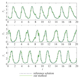
In Fig. 1 we show one sample path of $y_{a}, y_{b}$, and $y_{c}$ produced by our method. It can be seen that the numerical solution is positive and bounded, coinciding well with the reference exact solution of system (16). Hereby we take $h=10^{-3}$, and the exact solution is approximated by applying the midpoint method to system (16) with tiny time step $10^{-5}$.

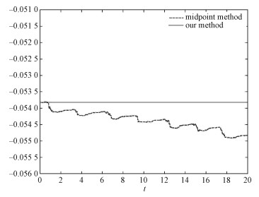
Figure 2 shows the evolution of the Casimir function with respect to $t$ produced by our method and the midpoint method directly applied to the system (16). Clearly our method can exactly preserve the Casimir function, while the midpoint method fails to preserve the Casimir function. Parameters here are the same with those for Fig. 1.

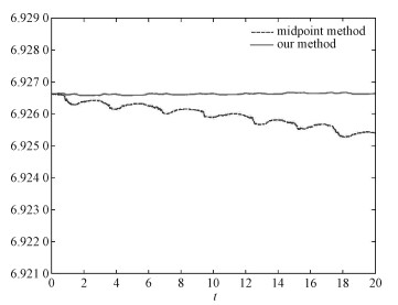
Figure 3 illustrates the evolution of the Hamiltonian $H(\boldsymbol{y})$ of the system (16) produced by our method and the midpoint method. It can be seen that our method can nearly preserve the Hamiltonian function of the system, while the midpoint method produces much larger error in the Hamiltonian evolution. Parameters are the same with those for Fig. 1.

Finally, Fig. 4 shows that our method is of root mean-square convergence order 1, coinciding with the theoretical result in Theorem 2.2. Hereby $h=$ $\left[2^{-11}, 2^{-10}, 2^{-9}, 2^{-8}, 2^{-7}\right]$, and 500 sample paths are taken to approximate the expectation. Other parameters are the same with those for Fig. 1.

4 Conclusion

We propose a numerical algorithm based on the Darboux-Lie theorem and the midpoint method for a class of stochastic Poisson systems, which can preserve both the Poisson structure and the Casimir functions of the original systems. We also prove that the proposed method has root mean-square convergence order 1. Numerical tests verify the theoretical results and illustrate the effectiveness of the method.