Opportunistic routing (OR)[1-3] has been an efficient routing strategy to improve the performance of a wireless multihop network. It takes advantage of the broadcast nature of the wireless medium and makes routing decisions by choosing next relay node among a group of the forwarder list in an online manner. Energy consumption is also a crucial issue in the study of a wireless multihop network to achieve balanced energy consumption and thus prolonged network lifetime. However, most existing opportunistic routing algorithms in the literature fail to consider the optimal trade-off between the routing performance and energy consumption in dynamic wireless environment[4]. It is thus highly desirable to design efficient opportunistic routing algorithm which can learn energy efficient routing policy in-telligently as needed.
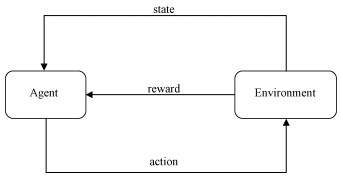
Reinforcement learning (RL)[5] is a classic machine learning method for solving sequence decision problems and has been widely used in image processing, natural language processing and also wireless environments for improved network performance. The basic framework of RL is shown in Fig. 1. Agent with decision-making capabilities constantly interacts with the environment to imple-ment the learning process. However, traditional RL methods are not scalable in many complex real-world applications. Such scalability issue could be addressed by combining the deep neural networks and RL into deep reinforcement learning (DRL) methods. With the generalization ability and feature extraction ability of deep neural networks, DRL has achieved breakthroughs in many fields, e.g., AlphaGo in the field of man-machine rivalry[6], automatic navigation[7] and machine translation[8], etc.
|
Download:
|
|
Fig. 1 Reinforcement learning framework |
|
Recently, RL has been a promising technique for improving the performance of wireless networks[9]. However, existing research on the routing and DRL in the field of wireless multihop networks are mostly conducted independently, which largely limits DRL's potential to improve the performance of wireless network. In-depth analysis are needed to exploit the potentials of DRL in wireless networks. For this purpose, in this paper, we propose an opportunistic deep Q-network (ODQN) routing algorithm for wireless multihop networks, which is designed to optimize the routing and energy consumption performance intelligently by joint design and optimization of the opportunistic routing and DRL technology. The major work and contributions of this paper are given as follows:
1) We formulate the opportunistic routing problem in wireless multihop networks as a Markov decision process and define the corresponding state space, action space, and reward function.
2) We propose a new energy efficient opportunistic routing algorithm using DRL to solve packet routing problem in wireless multihop networks, which can balance the routing perfor-mance and energy consumption effectively. The proposed algorithm can effectively alleviate the cold start problem in the traditional DQN based algorithm and improve the performance at the early stage of the learning.
3) Extensive simulations are conducted and the results show that the proposed algorithm demon-strates appreciable gain as compared with existing work.
1 Related workTraditional routing protocols developed for wireless multihop networks can be divided into the following four types: 1) routing-table-based proactive protocols like DSDV[10] and OLSR[11], 2) on-demand protocols like AODV[12], DSR[13], 3) hybrid routing protocols like ZRP[14], and 4) opportunistic routing protocols like ExOR[1], MORE[2], GeRaF[3].
Recently, some RL based routing algorithms have been proposed. Q-routing, proposed by Boyan and Littman[15], uses the Q-learning[16] algorithm to achieve adaptive routing. The simulation results indicated that Q-learning is effective under time varying network load level, traffic patterns and topologies. However, Q-routing, as well as its variants, e.g., predictive Q-routing[17] and dual Q-routing[18], has obvious disadvantages in wireless networks-They need to maintain a large Q-table and are not scalable to large state space. In Ref. [19], a reinforcement learning-based opportunistic routing (RLOR) algorithm has been proposed for providing live video streaming services over multi-hop wireless networks, which could effectively achieve a proper tradeoff between the transmission reliability and latency. By designing a distributed energy-efficient RL based routing algorithm for the wireless mesh IoT networks, Ref. [20] achieves considerable improvements in power efficiency, failure rate, and spectrum use efficiency.
Compared with the above traditional "shallow" RL based algorithms, DRL based algorithms, which takes advantage of deep neural networks[21] to improve the performance of RL[22], has been investigated in the area of wireless networks. Authors of Ref. [23] presented a distributed routing approach based on multi-agent RL which could simultaneously optimize the travel time of routed entities and energy consumption. Valadarsky et al.[24] applied DRL for network routing and showed that learning from the historical routing schemes with the consideration of the demand matrix and link utilization provides an efficient approach to smartly choose the optimal routing structure for future data forwarding. A DRL method proposed by Stampa et al.[25] optimizes the routing performance in SDN with the aim of reducing transmission delay. The experimental results show that there is significant improvement on transmission delay over various traffic intensities. Although existing work employ DRL to facilitate network routing in various environments, none of them consider both routing performance and network lifetime simultaneously under lossy wireless network environment.
2 Network model and problem formualtionIn this section, we formulate the energy efficient wireless opportunistic routing problem as a Markov decision process (MDP).
A.System model
We model a wireless multihop network with N nodes as a graph G=(V, E), where each vertex v ⊆ V represents a node, and every edge e ⊆ E represent a link between a pair of nodes. Each node could be served as the source node or destination node. When a packet p from source nodes s ⊆ V being sent towards its destination d ⊆ V arrives at a node j, it will be processed as follows:
· If j=d, then the packet has arrived its destination and this packet's process terminates successfully.
· Otherwise, the packet has been forwarded to an intermediate next hop, as chosen according to the learnt routing policy, which will be illustrated in Section IV.
When a node has packets to send or in its queue, it is treated as in the working state and each transmission will consume certain energy. Otherwise, the node has no energy consumption. When the energy of a node is lower than a given threshold, the node is treated as inactive and unreachable.
B.Problem formulation
We model the energy efficient opportunistic routing problem in wireless multihop networks under the centralized RL formulation, where a central agent is assumed to be responsible for learning the routing policy and chooses the action for each node according to the global state. We formulate the optimization of energy efficient opportunistic routing as an MDP defined by a tuple (S, A, P, R), where S is a finite set of states, A is a finite set of actions, P is a transition probability from state st to state st+1 after the agent taking action at at time slot t, and R is the immediate reward obtained after action at is performed indicating how good the current action is in the immediate sense.
Next, to formulate the above problem as an MDP, we give the details of the related observation space, action space, and reward function as follows.
1) State space
S: The state space. st={st1, …, stN}⊆S represents the joint network state at time slot t, which consists of the state obtained from each node according to their local information. The state of a node i∈V is denoted as sti={Dti, Bti, Eti}, where Dti=d is the destination of node i's current forwarding packet, Bti is the number of packets queued in node i, and Eti is the residual energy of node i, respectively.
2) Action space
A: The action space. A joint action at={at1, …, atN}⊆A at time slot t represents the action chosen by agent for all nodes to execute. ati=j⊆N means node j is chosen to forward current packet.
3) Reward
R: The reward rt(st, at) at time slot t is the immediately reward that agent can get when performing joint action at with the state transiting from st to st+1. It is defined as a function of the average packet transmission time and the residual energy as follows
| $ \begin{array}{l} r_t^i\left( {s_t^i, a_t^i} \right) = \\ \left\{ \begin{array}{l} \begin{array}{*{20}{l}} {0, }&{{\rm{if}}{\kern 1pt} {\kern 1pt} a_t^i{\kern 1pt} {\kern 1pt} {\rm{is destination}}}\\ { - 1, }&{{\rm{if}}{\kern 1pt} {\kern 1pt} a_t^i{\kern 1pt} {\kern 1pt} {\rm{is invalid neighbor}}} \end{array}\\ \begin{array}{*{20}{l}} {{f_c} + \frac{1}{{ET{X_{j, d}}}}\left( {{w_1}\frac{1}{{{{t'}_{i, j}}}} + {\rm{ }}{w_2}{{e'}_j} + \beta {P_j}} \right), {\kern 1pt} }&{{\rm{otherwise}}.} \end{array} \end{array} \right. \end{array} $ | (1) |
where rti(sti, ati) is the individual reward for each node, then the joint reward is defined as
| $ {r_t}\left( {{s_t}, {a_t}} \right) = \frac{1}{N}\sum\nolimits_{i = 1}^N {r_t^i} . $ | (2) |
If ati is the destination, then the packet has reached its target node and the transmission for this packet is finished. If ati is not the neighbor node of node i, a negative error reward will be given as the penalty. fc is a constant function that guarantee the reward function is non-negative. ETXj, d is the expected transmission count[26] from node j to a given destination node d calculated by summing up the ETX value along the shortest path from j to d chosen by Dijkstra algorithm[27]. t′i, j and e′j are the z-score values[28] of ti, j and ej for all nodes at time slot t for normalization.
4) Problem definition
By defining the state and action space and the reward, we can then formally formulate energy efficient opportunistic routing problem as the MDP. The objective of DRL algorithm is to find the deterministic optimal policy π* to maximizes the total accumulated reward rt(st, at). Thus, based on the formulations above, we define the problem of DRL based energy efficient opportunistic routing as maximization of the cumulative future reward:
| $ {G_t} = {r_t} + \gamma {r_{t + 1}} + {\gamma ^2}{r_{t + 2}} + \cdots . $ | (3) |
Our objective is to learn an optimal policy π* to route each packet correctly while maximizing the network lifetime, which has been proved to be NP-hard[29]. This makes it necessary to explore alternative solutions with the aim of maximizing the performance. In this paper, we explore the potential of the DRL to find the optimal energy efficient opportunistic routing policy. In the next section, we propose the ODQN-Routing algorithm for solving this problem.
3 ODQN-RoutingIn this section, we propose the ODQN-Routing algorithm, which can adapt to the dynamic changes of wireless medium and network topology to optimize the network routing and energy use performance by adjusting the routing policy intelligently.
A. Algorithm overview
Our proposed ODQN-Routing is based on the deep Q-network (DQN)[30], which transforms the Q-table update process into a function fitting problem in high-dimensional state-action space.
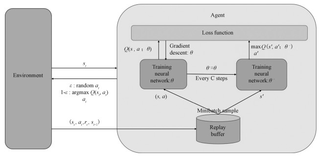
We assume a centralized ODQN agent which is responsible for interacting with the environment and learning the policy. Moreover, we assume that there exists a separate control channel, which could be used to collect and distribute control information directly between the centralized agent and each node in the network, an assumption made in a lot of existing DRL algorithms in this area. The framework of the ODQN agent is shown in Fig. 2. The agent observes the network information and gets the current network state st, selects an joint action at for all nodes according to the learnt policy with the ε-greedy principle, which randomly selects neighbor nodes as the next hop with a probability of ε, and selects the next hop node with the largest Q value with a probability of 1-ε. Then the agent gets the reward rt(st, at), and enters the next state st+1. The experience tuple (st, at, rt, st+1) is stored in the replay buffer. In the training phase, a small batch of state transition pair samples are randomly extracted from the replay buffer to train the ODQN agent.
|
Download:
|
|
Fig. 2 ODQN agent framework |
|
B.ODQN agent training
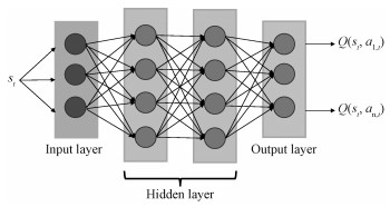
The neural network architecture of our ODQN-Routing agent is shown in Fig. 3, which has one input layer, two fully connected hidden layers and one output layer. Let θ denote the training neural network parameters, and θ- denote the target neural network parameters. ODQN agent tries to minimize the loss function defined as the difference between the target value and the estimated value.
| $ {L_{{\rm{DQN}}}}\left( \theta \right) = E\left[ {{{\left( {y - Q\left( {s, a;\theta } \right)} \right)}^2}} \right]. $ | (4) |
|
Download:
|
|
Fig. 3 Neural network structure in ODQN-Routing |
|
where y is the target value denoted as
| $ y = r + \gamma \mathop {{\rm{max}}}\limits_{a\prime } Q\left( {s\prime , a\prime ;{\theta ^ - }} \right). $ | (5) |
The gradient descent method is used to update the parameters with learning rate α.
| $ {\nabla _\theta }{L_{{\rm{DQN}}}}\left( \theta \right) = E\left[ {\left( {y - Q\left( {s, a;\theta } \right)} \right){\nabla _\theta }Q\left( {s, a;\theta } \right)} \right]. $ | (6) |
| $ \theta \leftarrow \theta + \alpha {\nabla _\theta }{L_{{\rm{DQN}}}}\left( \theta \right). $ | (7) |
The parameters of the training neural network are copied to the target neural network every C steps, and then the parameters of the target neural network are updated.
C.Cold start alleviation
There usually will be a cold start problem[31] for DRL based algorithm in real-world application as DRL requires huge amount of data before reaching acceptable performance. Thus, its performance could be compromised as the performance of RL during the learning process could be extremely poor due to its trial-and-error nature.
Therefore, to alleviate the cold start problem, we adopt the pre-training mechanism as in Ref. [31] in our proposed ODQN-Routing algorithm to speed up the agent's learning speed at the beginning phase. We use demonstration data as the starting policy to pre-train the agent so that it could perform well at the start of learning, and then let the agent interact with the environment to continue improving the routing performance by using its own collected data. In this paper, the demonstration data is collected by the AODV protocol to pre-train the agent to accelerate the learning process.
D.Proposed ODQN-Routing algorithm
The detailed ODQN-Routing algorithm is given in Algorithm 1, which can be divided into two phases: pre-training and policy learning.
Initialization: In line 1, we collect the demonstration data of AODV and store such data in the demonstration data buffer
Pre-training phase: From line 2 to line 8, before starting interaction with the environment, we perform k steps pre-training phase by sampling the mini-batch tuples from demonstration data buffer
| $ {L_{{\rm{pre}}}} = {L_{{\rm{DQN}}}} + {\gamma _1}{L_s} + {\gamma _2}{L_2}. $ | (8) |
where γ1, γ2 are parameters that regulate the weight between Ls and L2.Lpre is defined as the combination of the DQN loss LDQN in (3), the supervised large margin classification loss Ls, and the L2 regulari-zation loss on the neural network's weights and biases to prevent overfitting on the demonstration data. The supervised loss Ls is defined as
| $ {L_s} = \mathop {{\rm{max}}}\limits_a \left[ {Q\left( {s, a} \right) + l\left( {{a_e}, a} \right)} \right] - Q\left( {s, {a_e}} \right). $ | (9) |
| $ l\left( {{a_e}, a} \right) = \left\{ {\begin{array}{*{20}{L}} {0, }&{a = {a_e}}\\ {1, }&{{\rm{otherwise}}} \end{array}} \right.. $ | (10) |
where ae is the action from the demonstration data.
Then the loss function Lpre is minimized using the gradient descent optimizer. The target neural network's parameters θ- is updated by θ every C steps. The purpose of pre-training phase is to make the agent learn the starting policy from the demon-stration data to gain better initial performance.
Policy learning phase: Once k steps pre-training is completed, the agent enters the policy learning phase to interact with the environment to learn its own policy as in lines 9-23. From line 11 to line 14, the agent collects the information and get the state st, chooses action at, receives reward rt, and enters next state st+1. The self-generated data tuple (st, at, rt, st+1) will be added into replay buffer
Algorithm 1. ODQN-Routing algorithm
1: Initialization:
Initialize the training neural network's parameters θ and target neural network's parameters θ-, replay buffer
2: Pre-training:
3: for t = 1, 2, …, k do
4: Sample n tuples in demonstration data buffer
5: Calculate loss function Lpre using target neural network.
6: Use gradient descent to update the parameters of the training neural network: θ←θ+αΔθLpre.
7: Update the target neural network's parameter θ- every C steps: θ-←θ.
8: end for
9: Policy learning:
10: for t = 1, 2, …, do
11: The agent gets the state st.
12: Select ε-greedy action at.
13: Get the reward rt and enter the next state st+1.
14: Store (st, at, rt, st+1) into replay buffer
15: Sample n tuples from
16: Calculate loss function Lpre using target neural network: demonstration data use Lpre, self-generated data use LDQN.
17: Use gradient descent to update the parameters of the training neural network.
18: Update target neural network's parameters every C steps: θ-← θ.
19:
if η>0 then
20:
η←η-τ
21:
else
22:
η←0
23:End for
In this section, we conduct extensive simulations to evaluate the performance of ODQN-Routing algorithm by comparing it with existing work.
A.Simulation environment
We used Python 3.6 to build the event-driven simulator and used TensorFlow as the deep learning framework to implement DRL based routing. We built the wireless multihop network environment on the basis of Networkx[32]. In the simulations, we implemented the following algorithms for comparison purpose: (a) The proposed ODQN-Routing algorithm, (b) AODV algorithm, (c) Q-Routing algorithm, and (d) ODQN-Routing algorithm without pre-training, referred to as DQN-Routing.
In the simulations, we implemented the simulation experiments with 10, 20, 30, 40, 50 nodes in the network, respectively, and each node has a random number of neighbor nodes. Each simulation lasts for 2 500 s. Each reported result was averaged over 50 tests, each of which was due to a different random network topology. The bandwidth of each link in the wireless network under simulations was randomly set among 1, 2, 5.5, and 11 Mbit/s. The packet generation rate is subject to a Poisson distribution with the mean value of 10 packets per second and the packet size is set to 1 000 bytes with randomly generated source node and destination node. The queue length of each node is set to 500 packets. We used 1 000 packets based on AODV to pre-train the neural networks for 500 steps. The parameter settings in our simulations are shown in Table 1, where the settings related to deep Q-learning were also used in Refs. [31, 33].
|
|
Table 1 Parameter settings |
In the simulations, the initial energy of each node was set to 1 Joule. The transmit energy for packet transmission is 50 nJ/bit and that for processing queued packets is 40 nJ/bit. Moreover, when the residual energy of a network node is less than half of the mean residual energy of nodes in the network, it is treated as an inactive node and will be temporally removed from the network topology for any routing operations.
In the simulations, we compared the performance of different algorithms in terms of following measures:
Average packet transmission time
| $ \frac{1}{{\left| P \right|}}\sum\nolimits_{p \in P} {{t_p}} . $ | (11) |
We define tp as the total transmission time from the source to destination node of packet p ∈ P, P is the set of packets in the network and |P| is the total number of packets.
Network lifetime
| $ \frac{{{N_{{\rm{active}}}}}}{{\left| V \right|}}. $ | (12) |
We use the proportion of active nodes remaining in the network to characterize the network lifetime, where Nactive is the number of active nodes in the network when the simulation terminates and |V| represents the network size.
Average path length
| $ \frac{1}{{\left| P \right|}}\sum\nolimits_{p \in P} {{L_p}} . $ | (13) |
where Lp is the path length of packet p ∈ P.
Packet loss rate
| $ \frac{{{D_n}}}{{\left| P \right|}}. $ | (14) |
where Dn is the number of packets that fail to reach their destinations.
B.Simulation results
Average transmission time: Figure 4 shows the variation of average packet transmission time of different algorithms. It can be seen that at the beginning of the simulation, the average packet transmission time of Q-Routing and DQN-Routing are much larger than the other two algorithms. That is because the agent is in the process of policy learning and explores routing path through continuous trials and errors. Thus the reward obtained is unstable. In contrast, as the ODQN-Routing allows pre-training the agent using demonstration data from AODV, the routing policy can be optimized much more quickly. It can also be seen that during the training process, the transmission time of ODQN-Routing and DQN-Routing can both cover to a lower level than the traditional reinforcement learning routing algorithm Q-Routing. In general, the transmission time by ODQN-Routing is 50.1% shorter than that by Q-Routing, and 30.2% shorter than that by DQN-Routing. The results can verify that ODQN-Routing can significantly improve the average transmission time performance.

|
Download:
|
|
Fig. 4 Comparison of average transmission time |
|
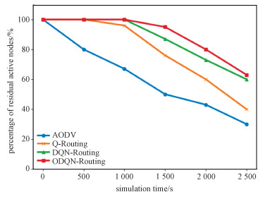
Network lifetime: Figure 5 compares the network lifetime performance of different algorithm. In Fig. 5, at the beginning of simulations, the percentage of active nodes by ODQN-Routing, Q-Routing, and DQN-Routing are quite similar as all nodes have high level residual energy at this moment. As the simulations elove, ODQN-Routing and DQN-Routing allow the ODQN agent to fully train and learn optimalized routing policy through DRL technology to adaptively select the nexthops to avoid rapid depletion of nodes in the network. Specifically, ODQN-Routing prolongs the network lifetime by 57.1% as compared with Q-Routing and 10.7% as compared with DQN-Routing algorithm. In the simulations, the value of w2 was set to 0.93 to effectively balance the energy consumption while reducing packet transmission time.
|
Download:
|
|
Fig. 5 Comparison of average network lifetime |
|
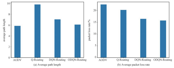
Average path length: Figure 6 (a) compares the average path length performance of different algorithms. The results show that the average path length by ODQN-Routing is shorter than that by Q-Routing and DQN-Routing. As compared with Q-Routing, ODQN-Routing could effectively reduce the average path length by up to 40.1%, indicating that ODQN-Routing could learn more effective routing poliy by considering the ETX values to destinations when making packet forwarding decisions, which could effectively avoid the detouring of the data packets to longer paths. The average path length by ODQN-Routing is 13.8% shorter than that by DQN-Routing, indicating the use of demostration data for the agent pre-training can significantly improve the learning efficiency, which enables the agent to learn optimalized routing policy faster.
|
Download:
|
|
Fig. 6 Comparison of average path length and average packet loss rate |
|
Packet loss rate: Figure 6 (b) compares the packet loss rate performance of different algorithms. In Fig. 7, it is seen that ODQN-Routing outperforms other algorithms in terms of packet loss rate. Moreover, ODQN-Routing can reduce the packet loss rate by 30.1% and 24.8% as compared with AODV and Q-Routing, respectively.
5 ConclusionIn this paper, we investigated how to improve the energy efficiency by applying DRL based routing in wireless multihop network. Regarding this, a formulation of energy efficient opportunistic routing was built as an MDP problem. To address the problem, we first defined the corresponding state space, action space, and reward function, and then proposed the ODQN-Routing algorithm. Extensive simulations were conducted and the results demonstrate that the proposed algorithm yields better performance as compared with existing work. Our work demonstrates that DRL based routing has significant advantages in improving the routing performance of wireless networks. In the future, we shall consider how to combine inverse reinforcement learning with wireless routing to strengthen the routing intelligence by learning more intrinsic reward functions. We also plan to design a full decentralized multi-agent reinforcement learning based algorithm for enabling efficient distributed routing in wireless multihop networks.
| [1] |
Biswas S, Morris R. Opportunistic routing in multi-hop wireless networks[J]. ACM SIGCOMM Computer Communication Review, 2004, 34(1): 69-74. DOI:10.1145/972374.972387 |
| [2] |
Chachulski S, Jennings M, Katti S, et al. Trading structure for randomness in wireless opportunistic routing[J]. ACM SIGCOMM Computer Communication Review, 2007, 37(4): 169-180. DOI:10.1145/1282427.1282400 |
| [3] |
Zorzi M, Rao R R. Geographic random forwarding (GeRaF) for ad hoc and sensor networks: energy and latency performance[J]. IEEE Transactions on Mobile Computing, 2003, 2(4): 349-365. DOI:10.1109/TMC.2003.1255650 |
| [4] |
Chu M, Li H, Liao X, et al. Reinforcement learning-based multiaccess control and battery prediction with energy harvesting in IoT systems[J]. IEEE Internet of Things Journal, 2019, 6(2): 2009-2020. DOI:10.1109/JIOT.2018.2872440 |
| [5] |
Sutton R S, Barto A G. Reinforcement learning: an introduction[M]. Cambridge, MA, USA: MIT press, 2018.
|
| [6] |
Silver D, Huang A, Maddison C J, et al. Mastering the game of Go with deep neural networks and tree search[J]. Nature, 2016, 529(7587): 484-489. DOI:10.1038/nature16961 |
| [7] |
Mirowski P, Pascanu R, Viola F, et al. Learning to navigate in complex environments[EB/OL]. ArXiv Preprint, 2016: 1611.03673. (2017-01-13)[2020-04-18]. http://arxiv.org/abs/1611.03673.
|
| [8] |
He D, Xia Y C, Qin T, et al. Dual learning for machine translation[C]//Advances in Neural Information Processing Systems, 2016: 820-828.
|
| [9] |
Mammeri Z. Reinforcement learning based routing in networks: review and classification of approaches[J]. IEEE Access, 2019, 7: 55916-55950. DOI:10.1109/ACCESS.2019.2913776 |
| [10] |
Perkins C E, Bhagwat P. Highly dynamic destination-sequenced distance-vector routing (DSDV) for mobile computers[J]. ACM SIGCOMM Computer Communication Review, 1994, 24(4): 234-244. DOI:10.1145/190809.190336 |
| [11] |
Jacquet P, Muhlethaler P, Clausen T, et al. Optimized link state routing protocol for ad hoc networks[C]//Proceedings of IEEE International Multi Topic Conference (IEEE INMIC 2001). Technology for the 21st Century. December 30, 2001, Lahore, Pakistan. IEEE, 2001: 62-68. DOI: 10.1109/INMIC.2001.995315.
|
| [12] |
Perkins C E, Royer E M. Ad-hoc on-demand distance vector routing[C]//Proceedings WMCSA'99. Second IEEE Workshop on Mobile Computing Systems and Applications. February 25-26, 1999, New Orleans, LA, USA. IEEE, 1999: 90-100. DOI: 10.1109/MCSA.1999.749281.
|
| [13] |
Park V D, Corson M S. A highly adaptive distributed routing algorithm for mobile wireless networks[C]//Proceedings of INFOCOM'97. April 7-11, 1997, Kobe, Japan. IEEE, 1997, 3: 1405-1413. DOI: 10.1109/INFCOM.1997.631180.
|
| [14] |
Youssef M, Ibrahim M, Abdelatif M, et al. Routing metrics of cognitive radio networks: a survey[J]. IEEE Communications Surveys & Tutorials, 2014, 16(1): 92-109. DOI:10.1109/SURV.2013.082713.00184 |
| [15] |
Boyan J, Littman M. Packet routing in dynamically changing networks: a reinforcement learning approach[C]//Advances in Neural Information Processing Systems, 1994: 671-678.
|
| [16] |
Watkins C J C H, Dayan P. Q-learning[J]. Machine learning, 1992, 8(3/4): 279-292. DOI:10.1007/BF00992698 |
| [17] |
Choi S P M, Yeung D Y. Predictive Q-routing: a memory-based reinforcement learning approach to adaptive traffic control[C]//Advances in Neural Information Processing Systems. 1996: 945-951.
|
| [18] |
Kumar S, Miikkulainen R. Dual reinforcement Q-routing: an on-line adaptive routing algorithm[C]//Proceedings of the Artificial Neural Networks in Engineering Conference, 1997: 231-238.
|
| [19] |
Tang K X, Li C L, Xiong H K, et al. Reinforcement learning-based opportunistic routing for live video streaming over multi-hop wireless networks[C]//2017 IEEE 19th International Workshop on Multimedia Signal Processing (MMSP). October 16-18, 2017, Luton, UK. IEEE, 2017: 1-6. DOI: 10.1109/MMSP.2017.8122255.
|
| [20] |
Liu Y, Tong K F, Wong K K. Reinforcement learning based routing for energy sensitive wireless mesh IoT networks[J]. Electronics Letters, 2019, 55(17): 966-968. DOI:10.1049/el.2019.1864 |
| [21] |
Zhao X D, Yang H J, Zong G D. Adaptive neural hierarchical sliding mode control of nonstrict-feedback nonlinear systems and an application to electronic circuits[J]. IEEE Transactions on Systems, Man, and Cybernetics: Systems, 2017, 47(7): 1394-1404. DOI:10.1109/TSMC.2016.2613885 |
| [22] |
Luong N C, Hoang D T, Gong S M, et al. Applications of deep reinforcement learning in communications and networking: a survey[J]. IEEE Communications Surveys & Tutorials, 2019, 21(4): 3133-3174. DOI:10.1109/COMST.2019.2916583 |
| [23] |
Mukhutdinov D, Filchenkov A, Shalyto A, et al. Multi-agent deep learning for simultaneous optimization for time and energy in distributed routing system[J]. Future Generation Computer Systems, 2019, 94: 587-600. DOI:10.1016/j.future.2018.12.037 |
| [24] |
Valadarsky A, Schapira M, Shahaf D, et al. A machine learning approach to routing[EB/OL]. ArXiv Preprint, 2017: 1708.03074. (2017-11-11)[2020-04-18]. http://arxiv.org/abs/1708.03074.
|
| [25] |
Stampa G, Arias M, Sánchez-Charles D, et al. A deep-reinforcement learning approach for software-defined networking routing optimization[EB/OL]. ArXiv Preprint, 2017: 1709.07080. (2017-09-20)[2020-04-18]. http://arxiv.org/abs/1709.07080.
|
| [26] |
de Couto D S J, Aguayo D, Bicket J, et al. A high-throughput path metric for multi-hop wireless routing[C]//Proceedings of the 9th Annual International Conference on Mobile Computing and Networking. 2003: 134-146. DOI: 10.1145/938985.939000.
|
| [27] |
Cormen T H, Leiserson C E, Rivest R L, et al. Introduction to algorithms[M]. Cambridge, MA, USA: MIT Press, 2009.
|
| [28] |
Jain A, Nandakumar K, Ross A. Score normalization in multimodal biometric systems[J]. Pattern Recognition, 2005, 38(12): 2270-2285. DOI:10.1016/j.patcog.2005.01.012 |
| [29] |
Wang Z, Crowcroft J. Quality-of-service routing for supporting multimedia applications[J]. IEEE Journal on Selected Areas in Communications, 1996, 14(7): 1228-1234. DOI:10.1109/49.536364 |
| [30] |
Mnih V, Kavukcuoglu K, Silver D, et al. Human-level control through deep reinforcement learning[J]. Nature, 2015, 518(7540): 529-533. DOI:10.1038/nature14236 |
| [31] |
Hester T, Vecerik M, Pietquin O, et al. Deep Q-learning from demonstrations [C]//Proceedings of the AAAI Conference on Artificial Intelligence, 2018, 32(1): 3223-3230.
|
| [32] |
Hagberg A, Swart P, S Chult D. Exploring network structure, dynamics, and function using NetworkX[C]//Proceedings of the 7th Python in Science Conference (SciPy). 2008: 11-15.
|
| [33] |
Du Y H, Xu Y, Xue L, et al. An energy-efficient cross-layer routing protocol for cognitive radio networks using apprenticeship deep reinforcement learning[J]. Energies, 2019, 12(14): 2829. DOI:10.3390/en1214829 |
 2022, Vol. 39


