


b. Landscape College of Beijing Forestry University, No.35 Qinghua East Road, Beijing 100083, China
Interactions between forest communities and ecosystems are reflected in species richness and abundance patterns (Wright, 2002). Distribution patterns of species richness and abundance are representative of community biodiversity and the structural characteristics and organization patterns of communities, which are important considerations in community ecology research (He and Gaston, 2000). Biodiversity has been shown to exert significant positive effects on ecosystem productivity. Species richness and abundance estimates vary significantly at different spatial scales, likely due to scale-dependent changes in ecological processes (Collins and Glenn, 1997; He et al., 2002; Giladi et al., 2011).
Although many theories have been proposed to explain variation in species diversity and species richness distribution patterns at different spatial scales (Silvertown and Law, 1987; Hacker and Gaines, 1997; Adler et al., 2007), it is still difficult to quantify their relative application. Many studies have found that neutral theory or niche theory best explains species richness and abundance patterns (MacArthur, 1957; Whittaker, 1972; Hubbell et al., 2001; Chase, 2003; Hubbell, 2005, 2006). Neutral theory proposes that the niche of each individual is equivalent (Hubbell et al., 2001; Chase, 2003), and has a certain scale effect. However, the simplicity of the neutral theory (e.g. the symmetric assumption) makes it vulnerable to criticism because it commonly contradicts reality (Lin et al., 2009). Niche theory proposes that niche differentiation, which is affected by available resources and environmental factors, is a necessary condition for species coexistence (Chase, 2003). A current goal of ecological studies is to reconcile neutral and niche theories by either incorporating neutral theory drift into niche theory or niche into the neutral theory framework (Hubbell, 2005, 2006).
Several models have been developed to assess the spatial distribution patterns of species richness and diversity. The Species Area Relationship Model (SAR) has been widely used to describe species richness distribution patterns (He et al., 2002; Fridley et al., 2006; Harte et al., 2009). However, SAR cannot be used to quantify the contributions of individual species to community species diversity. The Individual Species–Area Relationship model (ISAR) analyzes species richness and spatial patterns at the individual species level, and classifies species as accumulators, repellers, and neutral species (Wiegend et al., 2007). The Broken Stick Model and the Overlapping Niche Model are based on niche theory (Williams, 1964; Walker and Cyr, 2007). The Zero-sum Multinomial Model is derived from neutral theory. Statistical distributions that have been applied to these models, including lognormal and negative binomial distribution, have verified species richness and abundance patterns.
In this study, we used the Beijing Songshan Nature Reserve as a model system to identify mechanisms that influence the maintenance of species richness and abundance in an undisturbed forest. For this purpose, we used five models (a Log-Normal Model, a Broken Stick Model, a Zipf Model, a Niche Preemption Model, and a Neutral Model) to test which ecological processes best explained diversity and abundance patterns at six spatial scales. These models may also provide feasible suggestions for forest management.
2. Materials and methods 2.1. Study areaThis research was carried out in a 40-ha undisturbed pine forest in the Songshan Nature Reserve in northern China. The average annual temperature of the region is 8.5 ℃, with average daily temperatures ranging between 39 ℃ and -27.3 ℃. The mean duration of annual sunshine, cumulative rainfall, and evaporation are 2836.3 h, 493 mm, and 1770 mm respectively. The highest elevation of the Songshan Nature Reserve is 2198.39 m. Songshan Nature Reserve is home to 713 vascular plant species, 300 of which are medicinal plants; and 216 species of vertebrates, including 158 bird species. The dominant tree species within the study forest are Pinus tabuliformis Carrière, Fraxinus chinensis Roxb, Syinga reticulata var. Mandshurica, Quercus mongolica, Ulmus macrocarpa Hance and Juglans mandshurica.
2.2. Data collectionIn 2014, the 40-ha (400 m × 1000 m) study forest was established and divided into 1000 continuous 20 m × 20 m plots. The number of individual standing trees ≥1 cm diameter at breast height (dbh) were physically counted and measured at a height of 1.3 m above ground level. We recorded the spatial locations (GPS coordinates) of each plot and measured dbh and height of all free-standing trees at least 1 cm in diameter.
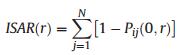
2.3. Data analysis 2.3.1. ISAR modelWe used an ISAR model to verify the effects of each individual species on species diversity at different spatial scales (0–50 m). ISAR is the expected number of species within a circular area of radius r around a randomly chosen individual of the target species i. The model is defined as:
|
where Pij (0, r) is the probability that species j is not present within r meters around any individual of the target species i (Wiegend et al., 2007). In order to quantify the significance of the effects of target species on species diversity, 95% confidence intervals were calculated by Complete Spatial Randomness (CSR). We used the null model to test the ISAR. When the empirically-determined ISAR(r) was larger than the second highest ISAR(r) of the 99 simulations of the null model at scale r, the species was regarded as a diversity accumulator (positive effect on species diversity) with an approximate significance level of 0.05. When the empirical ISAR(r) was smaller than the second smallest ISAR(r) of the 99 simulations at scale r, the species was classified as a diversity repeller (negative effect on species diversity) at scale r. Species were classified as neutral (no significant effect on species diversity) at scale r when the empirically-determined ISAR(r) was not outside of the null model range.
2.3.2. Species abundance sampling across spatial scalesIn order to quantify the ecological processes influencing species abundance distribution patterns at different spatial scales, we sampled species abundance within six area dimensions (10 m × 10 m; 0.01 ha, 20 m × 20 m; 0.04 ha, 40 m × 40 m; 0.16 ha, 60 m × 60 m; 0.36 ha, 80 m × 80 m; 0.64 ha, and 100 m × 100 m; 1 ha) or spatial scales. For each spatial scale, 600 randomly selected replicate areas were assessed.
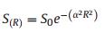
2.3.3. Species abundance distribution models 2.3.3.1. Log-Normal ModelThe Log-Normal Model (LNM), based on niche theory, was first proposed by Preston (1948). The model assumes that the logarithmic form of species abundance is normally distributed. The model is defined as:
|
(1) |
where S(R) is the number of species within the Rth octave to the left and right of the symmetrical curve; S0 is the number of species within the modal abundance octave and 1/a is the distribution width (Kevan and Belaoussoff, 1997).
2.3.3.2. Broken Stick ModelThe Broken Stick Model (BSM) was first proposed by MacArthur (1957). The sampled area is compared with a stick of unit length, S-1 points are placed at random, where S is area. The stick is broken at each point and the lengths of the S resulting segments are proportional to the abundances of S species. Assuming all species within the community share close taxonomic statuses and possess similar competitive capacities, the expected abundance of the ith rarest species among S species and N individual trees are:

|
(2) |
where k equals i. The model assumes that resource allocation among competitive species follows a one-dimensional gradient (Purves et al., 2005).
2.3.3.3. Zipf ModelThe Zipf Model (ZM) was first introduced by Frontier (1985), who assumed that species occupancy is dependent on the environmental and physical conditions and the species present. Cost of living is much higher for late successional species than for pioneer species. The abundance of the ith species is:

|
(3) |
where N is the number of individual trees, q is the predicted relative abundance of the species with the highest frequency within the community, and γ is a constant representing the average probability of species occupancy (Frontier, 1985).
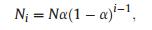
2.3.3.4. Niche Preemption ModelThe Niche Preemption Model (NPM) was proposed by Motomura (1932), who suggested that if a percent of the total niches is occupied by the most frequent species, then the second most frequent species occupies a(1-a) percent of the remaining niches. Accordingly, the niche occupied by ith species is a(1-a)i-1. The abundance of species is ranked according to the number of niches each species occupies. The expected abundance for the ith species is:
|
(4) |
where N is the total number of individual trees within the community (Motomura, 1932).
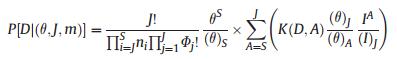
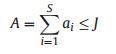
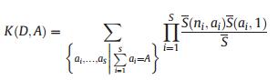
2.3.3.5. Neutral ModelThe Neutral Model (NM) was introduced by Hubbell (2001). Neutral theory makes the following two assumptions: (1) The total number of individual trees, regardless of species, within a specific community is constant; therefore, in a saturated community, an increase in number of individuals of one species will result, to some extent, in a decrease in number of individuals of another species. (2) Functional and physiological traits do not differ among species, such that neutral theory assumes all species have identical natality, mortality, immigration, and speciation rates. When these two assumptions are true, species abundance shows a zero-sum multinomial distribution. The probability distribution of species abundance follows the following equations:
|
(5) |

|
(6) |
|
(7) |
|
(8) |
where S is the total number of species, ns is the abundance of the sth species, and D = (n1, n2, n3 … ns) is the species abundance distribution. θ is an index representing the 'fundamental diversity'; the greater the magnitude of θ, the larger the number of species within a community. j is the total number of individual trees. Φ is the number of species with j individual trees. i is the number of individual trees that migrated into the local community. A is the number of individual trees of the parent generation and ai is the number of individual trees of the parent generation of the ith species. K(D, A) is a multinomial coefficient. Expected species abundance was estimated as the mean of 600 simulations of neutral communities using the estimated θ and m predicted by a maximum likelihood estimation method and the total number of observed individual trees j (Walker and Cyr, 2007).
2.3.3.6. Model evaluationAkaike Information Criterion (AIC) values were used to test for significant differences between the expected and observed species abundance distribution patterns. We also compared AIC values for the different models to identify the optimum model. The best model has a ΔAIC of zero. All models with a ΔAIC value of less than two are equally valid. All calculations were carried out in R 3.2.3 using the package 'vegan' and the package 'untb' (Hankin, 2007; Oksanen et al., 2009).
3. Results 3.1. Species richness patternsThe number of species detected was strongly influenced by the spatial scale. The number of species increased sharply when the area increased across small spatial scales; however, at larger spatial scales, the rate of increase in the number of species detected decreased when the scale increased (Fig. 1). Generally, when the spatial scale increased, the proportion of accumulators decreased and the proportion of neutral species and repellers increased. At small spatial scales (0–10 m), accumulators dominated forest communities. At large spatial scales (10–50 m), neutral species dominated, but repellers also accounted for a considerable proportion of forest communities. Accumulators and neutral species contributed to the majority of species diversity, but the relative importance of each species type was strongly influenced by spatial scale (Fig. 2).

|
| Fig. 1 Individual species–area curves of the studied species (e.g. Pinus). |

|
| Fig. 2 Variation in contributions of accumulators, neutral species, and repellers to diversity across spatial scales. Red lines represent accumulators, blue lines represent repellers, and black lines represent neutral species. |
The species abundance patterns within the 40-ha Pinus forest are presented in Fig. 3 and Table 1. At the 10 m × 10 m, 20 m × 20 m, and 40 m × 40 m scales, all models had a good fit to the observed species abundance patterns. At the 60 m × 60 m scale, the expected species abundance distributions modeled by the BSM (p < 0.01) and ZM (p < 0.01) were significantly different from the observed species abundance based on the chi-square test. At the 80 m × 80 m and 100 m × 100 m scale, only the NPM and NM passed the Chi-square test. A comparison of AIC values showed that NPM was the best-fit model with the lowest AIC values (-29.06 and -31.21, respectively) at the 10 m × 10 m and 20 m × 20 m scales. NM was the best model at the remaining spatial scales (AIC = -33.04, -28.45, -29.10, and -29.37). For the neutral model, the fundamental diversity index (θ) was unimodal across all spatial scales and the immigration rate (m) decreased with increasing spatial scale.

|
| Fig. 3 Observed and modeled species abundance distribution patterns based on six sampled spatial scales within the 40-ha undisturbed Pinus forest. |
| Sampling scale | θ | m | Testing method | BSM | NPM | LNM | ZM | NM |
| 10 m × 10 m | 3.30 | 1.7 × 10⁻¹ | AIC | -18.21 | -29.06 | -11.89 | -18.68 | -20.4 |
| ΔAIC | 6.23 | 0 | 7.45 | 6.12 | 4.97 | |||
| 20 m × 20 m | 3.22 | 3.8 × 10⁻² | AIC | -14.45 | -31.21 | -27.66 | -9.80 | -9.35 |
| ΔAIC | 7.01 | 0 | 4.56 | 8.52 | 9.34 | |||
| 40 m × 40 m | 3.14 | 9.6 × 10⁻³ | AIC | 4.32 | -16.82 | -7.86 | 9.37 | -33.04 |
| ΔAIC | 10.52 | 7.43 | 9.78 | 12.34 | 0 | |||
| 60 m × 60 m | 3.30 | 4.7 × 10⁻³ | AIC | 16.2 | -26.30 | 5.89 | 19.65 | -28.45 |
| ΔAIC | 9.87 | 2.35 | 6.78 | 11.23 | 0 | |||
| 80 m × 80 m | 3.58 | 2.9 × 10⁻³ | AIC | 20.70 | -23.40 | 9.31 | 24.97 | -29.10 |
| ΔAIC | 13.21 | 2.67 | 5.62 | 15.42 | 0 | |||
| 100 m × 100 m | 3.90 | 2.0 × 10⁻³ | AIC | 23.24 | -22.59 | 7.43 | 27.03 | -29.37 |
| ΔAIC | 12.32 | 6.34 | 8.79 | 14.34 | 0 | |||
| BSM, NPM, LNM, ZM and NM stand for Nroken Stick Model, Niche Preemption Model, Log-Normal Model, Zipf Model, and Neutral Model, respectively. θ and m are the parameters of neutral theory model. AIC stands for Akaike Information Criterion. ΔAIC of subsequent models is calculated as ΔAIC0 - ΔAICi, were 0 is the AIC value of the first model, and i is the AIC value of the next models. | ||||||||
Biodiversity has been shown to exert significant positive effects on ecosystem productivity; therefore, understanding the mechanisms underlying biodiversity maintenance is critical to forest management. Increased forest productivity can effectively improve the efficiency of material circulation (Liang et al., 2016). In this study, we fitted species richness and species abundance patterns with several models to identify the ecological processes involved in community construction as well as the relative contributions of these processes to the formation of species richness and abundance distribution patterns.
We found that accumulators and neutral species equally determined the local tree diversity within communities of an undistributed temperate Pinus forest. At small spatial scales (0–10 m), accumulators dominated forest communities. These findings support the niche theory, which proposes that species diversity is improved by variation in niche utilization among tree species (He and Duncan, 2000). Dominance of neutral species at larger spatial scales (10–50 m) supports the neutral theory, which proposes that community biodiversity construction is a result of neutral process (He and Legendre, 2002).
We compared fitted species abundance observations from our target forest to five species abundance models. All five models fit observations well at the two smallest sampling scales (10 m × 10 m and 20 m × 20 m), suggesting that both neutral and niche processes are important in structuring species abundance distribution patterns. We assumed density dependence would have a strong effect at small scales, resulting in competitive exclusion, and, consequently reduce interspecific density (Volkov et al., 2005). The community was affected by strong interspecific competition at small spatial scales. This type of competition improves species diversity by promoting niche differentiation (Aarssen, 1983). At the intermediate (40 m × 40 m and 60 m × 60 m) and large (80 m × 80 m and 100 m × 100 m) spatial scales, neutral model clearly matched observations, which suggests that the importance of neutral processes increase with spatial scale, although the contributions of niche processes cannot be ignored.
Author contributionsJ Gao and YH Liu designed the study; J Gao and YH Liu collected the data; J Gao, P Zhang and X Zhang performed analyses; J Gao led the writing; J Gao and YH Liu contributed substantially to revisions. J Gao and P Zhang are joint first authors.
Competing financial interestsThe authors declare no competing financial interests.
AcknowledgmentsThis work was supported by the Beijing Common Construction Project Research and demonstration on the regression technique of the minimum population of wild plants (2016YFC0503106). We would also like to thank Christine Verhille at the University of British Columbia for her assistance with English language and grammatical editing of the manuscript.
Aarssen L.W., 1983. Ecological combining ability and competitive combining ability in plants: toward a general evolutionary theory of coexistence in systems of competition. Am. Nat, 122, 707-731.
DOI:10.1086/284167 |
||
Adler P.B., Lamber J.H., Levine J.M., 2007. A niche for neutrality. Ecol. Lett, 10, 95-104.
DOI:10.1111/ele.2007.10.issue-2 |
||
Collins S.L., Glenn S.M., 1997. Effects of organismal and distance scaling on analysis of species distribution and abundance. Ecol. Appl, 7, 543-551.
DOI:10.1890/1051-0761(1997)007[0543:EOOADS]2.0.CO;2 |
||
Chase J.M., 2003. Community assembly: when should history matter?. Oecologia, 136, 489-498.
DOI:10.1007/s00442-003-1311-7 |
||
Frontier S., 1985. Diversity and structure in aquatic ecosystems. Oceanogr. Mar. Biol, 23, 253-312.
|
||
Fridley J.D., Peet R.K., van der Maarel E., et al., 2006. Integration of local and regional speciesearea relationships from spaceetime species accumulation. Am. Nat, 168, 133-143.
|
||
Giladi I., Ziv Y., May F., et al., 2011. Scale-dependent determinants of plant species richness in a semi-arid fragmented Agro-ecosystem. J. Veg. Sci, 6, 983-996.
|
||
Hacker S.D., Gaines S.D., 1997. Some implications of direct positive interactions for community species diversity. Ecology, 78, 1990-2003.
DOI:10.1890/0012-9658(1997)078[1990:SIODPI]2.0.CO;2 |
||
Hankin R.K.S., 2007. Introducing untb, an r package for simulating ecological drift under the unified neutral theory of biodiversity. J. Stat. Software, 22.
|
||
Harte J., Smith A.B., Storch D., 2009. Biodiversity scales from plots to biomes with a universal speciesearea curve. Ecol. Lett, 12, 789-797.
DOI:10.1111/ele.2009.12.issue-8 |
||
He F., Gaston K.J., 2000. Estimating species abundance from occurrence. Am. Nat, 156, 553-559.
DOI:10.1086/303403 |
||
He F., Duncan R.P., 2000. Density-dependent effects on tree survival in an old growth Douglas fir forest. J. Ecol, 88, 676-688.
DOI:10.1046/j.1365-2745.2000.00482.x |
||
He F., Legendre P., 2002. Species diversity patterns derived from speciesearea models. Ecology, 83, 1185-1198.
|
||
He F., Lafrankie J.V., Song B.O., 2002. Scale dependence of tree abundance and richness in a tropical rain forest, Malaysia. Landsc. Ecol, 17, 559-568.
DOI:10.1023/A:1021514104193 |
||
Hubbell S.P., Ahumada J.A., Condit R., et al., 2001. Local neighborhood effects on long-term survival of individual trees in a neotropical forest. Ecol. Res, 16, 859-875.
DOI:10.1046/j.1440-1703.2001.00445.x |
||
Hubbell S.P., 2001. The Unified Ueutral Theory of Biodiversity and Biogeography. Princeton University Press, Princeton and Oxford. |
||
Hubbell S.P., 2005. Neutral theory in community ecology and the hypothesis of functional equivalence. Funct. Ecol, 19, 166-172.
DOI:10.1111/fec.2005.19.issue-1 |
||
Hubbell S.P., 2006. The neutral theory and evolution of ecological equivalence. Ecology, 87, 1387-1398.
DOI:10.1890/0012-9658(2006)87[1387:NTATEO]2.0.CO;2 |
||
Kevan P.G., Belaoussoff S., 1997. Log-normality of biodiversity and abundance in diagnosis and measuring of ecosystemic health: pesticide stress on pollinators on blueberry heaths. J. Appl. Ecol, 34, 1122-1136.
DOI:10.2307/2405226 |
||
Lin K., Zhang D.Y., He F., 2009. Demographic trade-offs in a neutral model explain death-rate-bundance-rank relationship. Ecology, 90, 31-38.
DOI:10.1890/07-2079.1 |
||
Liang J.J., Crowther T.W., Picard N., et al., 2016. Positive biodiversity-productivity relationship predominant in global forests. Science, 354.
|
||
MacArthur R.H., 1957. On the relative abundance of bird species. Proc. Nat. Acad. Sci. U. S. A, 43, 293-295.
DOI:10.1073/pnas.43.3.293 |
||
Motomura I., 1932. On the statistical treatment of communities. Zool. Manag, 44, 379-383.
|
||
Oksanen, J., Kindt, R., O'Hara, B., et al., 2009. Vegan: Community Ecology Package. Version 1. 15. R Project for Statistical Computing, Vienna, Austria.
|
||
Preston F.W., 1948. The commonness, and rarity, of species. Ecology, 29, 254-283.
DOI:10.2307/1930989 |
||
Purves, D. W., Pacala, S. W., Burslem, D. F. R. P., et al., 2005. Ecological Drift in Nichestructured Communities: Neutral Pattern Does Not Imply Neutral Process.
|
||
Silvertown J., Law R., 1987. Do plants need niches? Some recent developments in plant community ecology. Trends Ecol. Evol, 2, 24-26.
DOI:10.1016/0169-5347(87)90197-2 |
||
Volkov I., Banavar J.R., He F., et al., 2005. Density dependence explains tree species abundance and diversity in tropical forests. Nature, 438, 658-661.
DOI:10.1038/nature04030 |
||
Walker S.C., Cyr H., 2007. Testing the standard neutral model of biodiversity in lake communities. Oikos, 116, 143-155.
DOI:10.1111/oik.2007.116.issue-1 |
||
Whittaker R.H., 1972. Evolution and measurement of species diversity. Taxon, 21, 213-251.
DOI:10.2307/1218190 |
||
Williams, C. B., 1964. Patterns in the Balance of Nature, and Related Problems in Quantitative Ecology.
|
||
Wright S.J., 2002. Plant diversity in tropical forests: a review of mechanisms of species coexistence. Oecologia, 130, 1-14.
DOI:10.1007/s004420100809 |
||
Wiegend T., Gunatilleke S., Gunatilleke N., et al., 2007. Species association in a heterogeneous Sri Lankan dipterocarp forest. Am. Nat, 170, 77-95.
DOI:10.1086/521240 |