


2. University of Bordeaux, IMB UMR 5251, INRIA Bordeaux Sud-Ouest, F-33400 Talence, France;
3. INRIA Bordeaux Sud-Ouest, F-33400 Talence, France
2. University of Bordeaux, IMB UMR 5251, INRIA Bordeaux Sud-Ouest, F-33400 Talence, France;
3. INRIA Bordeaux Sud-Ouest, F-33400 Talence, France
0 Introduction
When dealing with Computational Fluid Dynamics simulations,two kinds of grids are usually used: body-fitted grids and embedded ones. For body fitted grids,solid wall boundaries are meshed and boundary conditions (BCs) are applied on the wall according to additional equations (Neumann or Dirichlet BCs). On the contrary,immersed boundary methods (IBM) are characterised by a mesh covering the entire domain,and BCs are taken into account in a different way. The penalization technique [1] is an IBM in which the BCs are handled inside the equations by adding source terms. In this method,the solid body is located on the mesh by the 0 isovalue of the signed distance function. It is then necessary to define this isovalue as well as possible. Mesh adaptation is then introduced [2, 3, 4] to catch precisely this isovalue and to accurately compute the penalized source terms. We propose here to solve the penalized compressible Navier-Stokes equations on adapted grids using a residual distri-bution scheme. Those schemes [5, 6, 7, 8] are chosen for their easy order increase and parallelization. Penalization combined with mesh adaptation provides a good method to deal with moving bodies. Indeed,for a given (or computed) movement of the solid body,if the new position and a mesh can be provided,the solution at the new time step can be computed. In this work the penalization technique applied to anisotropic meshes,presented in [1],is extended in the framework of Residual Distribution Schemes (RDS). A methodology is proposed to account for unsteady flows and moving bodies. Again,in order to improve accuracy of the wall treatment we investigate a dynamic tracking of the moving interface. In [4],a methodology is proposed to follow the level-set function by advection and to get dynamic mesh adaptation. In this work,we propose to follow the process proposed in [4] and to track the surface interface with mesh adaptation.
1 Description of the MethodIBM methods are characterized by a mesh covering the entire domain. To take into account solid bodies inside the domain the first step consists in localizing the solids' interfaces (lines in two dimensions and surfaces in three dimensions). A common way for that is to use a level-set function that defines for each node of the mesh the distance between this node and the closest solid interface.
1.1 Signed Distance Function to a SolidFrom a practical point of view,the level-set function chosen in this work is the signed distance function (SDF). The SDF is the distance of the considered point to the solid surface with a sign in order to determine if the point is inside or outside the surface. For an inside point,the SDF is negative and for an outside one,the SDF is positive. One way of computing the SDF,see Dapogny and Frey [9],is to solve the unsteady Eikonal equation. The inside of the surface to model is defined by
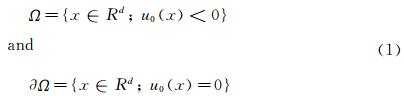
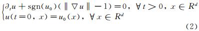
with d the dimension of space and u0 a continuous function. Then,the SDF can be considered as the solution of the following unsteady Eikonal equation:
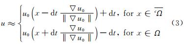
Using the method of characteristics,the following approached solution is then obtained by the system of Eq. (3):
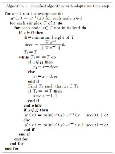
In order to be more accurate,the time step dt has been chosen using a local time stepping technique. Indeed,as the solution is “propagated” over the mesh,the idea is to chose one time step by element which allows to trace back the characteristic in the element “just below” which is already initialized (see Fig. 1). The minimum height (in the element) is used for the initialization of dt. Then,as long as 
 dt still belongs to the considered element,dt is increased (see Fig. 1). The algorithm proposed in [9] has been modified as follows in the algorithm (1).
 |
|
Fig. 1 Wanted arrival element while tracing back characteristics. Improvement of dt so as to have dt belonging to another element.
|
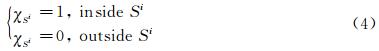
Once the SDF is defined over the domain,for each solid body Si the characteristic function of this solid,χSi can be defined such as
1.2 Penalized Navier-Stokes Equations
When a penalization technique is used as an immersed boundary method the solids around which the flow is computed are defined using the so-called penalization method or Brinckman-Navier-Stokes equations. Here,the solids are considered as porous media with a very small intrinsic permeability. The idea is then to extend the velocity field inside the solid body and to solve the flow equations with a penalization term to enforce rigid motion inside the solid. The sign distance function to the solid is used to capture the interface of the solid Si. The penalty terms are added to the classical Navier-Stokes equations to account for the solids inside the domain,as it is described in Eq. (5). We have
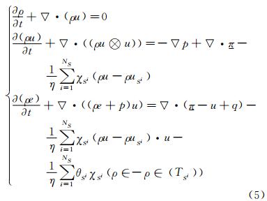
where ρ is the density,u is the velocity,p the pressure,π is the stress tensor and q the heat flux. NS corresponds to the number of solids considered inside the domain,χSi,Eq. (4),is the character-istic function of the solid Si,θ(Si) lets the possibility to penalize the energy (Dirichlet BC) or not (Neumann BC),and η is a parameter chosen small enough (1/η>>1). In addition of those equations,the variables are linked by an equation of state: in our case we consider the perfect gas law.
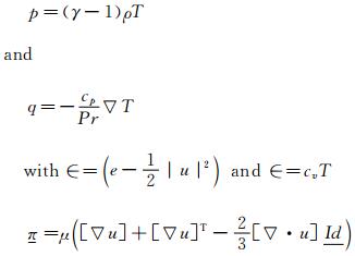
In these modified equations,the penalty terms are the terms,which include directly the boundary conditions of the solids in the equations. Indeed,outside the solids,the χSi functions are equal to 0 and so the penalization term vanishes and the usual Navier-Stokes equations are found back. On the opposite,inside a solid,the characteristic function is equal to one,and as 1/η is chosen large enough,the penalty terms dominate and the boundary values are imposed. The accuracy of the method depends on the value of η,in all simulations,we use an implicit scheme with η=1×10-12. This system can be formulated in a matrix way:
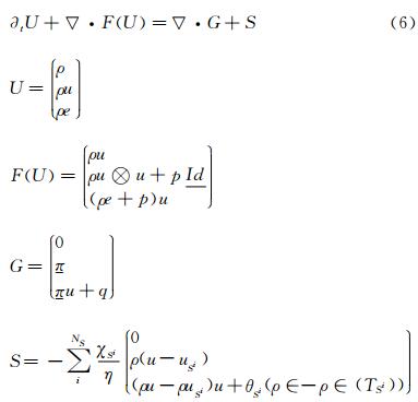
where U are the conservative variables,F and G are the advection and viscous flux and S the penalty source term.
1.3 Unstructured Mesh AdaptationOur numerical simulations are performed on unstructured anisotropic meshes (triangles in two dimensions and tetrahedra in three dimensions). In Abgrall et al. [1] we propose to combine our level-set based penalization approach to mesh adaptation. The idea is to conserve the simplicity of the embedded approaches for grid generation process and improve the accuracy of wall treatments by using mesh adaptation. Mesh adaptations are performed using two criteria,the signed distance function (interface of the solid body) and the velocity component of the flow solution. As explained in section 1.1,the solid is located on the mesh thanks to the SDF. In order to define as precisely as possible the solid,mesh adaptation with respect to the 0 level set function can be performed. Indeed,it allows refining the mesh close to the solid boundaries. Thus,the penalization is imposed in a rigorous way. In addition,anisotropic meshes are used. Those meshes are defined by the fact that elements (triangles or tetrahedra) can be stretched a lot,which allows inserting fewer elements in refined areas.
The aim in mesh adaptation is to find a good error estimator for a solution on a mesh. In [3, 4] metrics have been used to construct error estimator. Those metrics are positive definite symmetric matrices defined for each nodes of the mesh. The matrix contains the size and direction of the edges. Indeed,those matrices are diagonalizable,and the eigenvalues λi are linked to the sizes hi of the elements in the direction i(λi=1/hi2),those directions being given by the eigenvectors. To adapt with respect to the 0 level set,it is shown in [9] that the following metric can control the approximation of the SDF φ with an error ε:
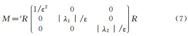
with R=(φ,v1,v2),where (v1,v2) is a base of the tangential plane of the surface defined by the isovalues of φ,and λi the eigenvalues of the Hessian of φ. This metric is imposed in a vicinity W of the surface (see Fig. 2).
 |
| Fig. 2 Area of fine mesh integration. |
Another important and useful way of using mesh adaptation is in areas of large physical variations. Indeed,it allows refining the mesh in order to better catch some phenomena. Thus,without increasing that much the number of nodes and elements,the solution can be considerably improved. For this kind of adaptation,the aim is to control the interpolation error between the exact solution u and its interpolant Ⅱhu on the mesh. It has been proved in [3] that an upper bound of this error on an element K is given by:
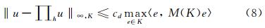
where e denote the edges of the mesh,cd is a constant depending on the dimension and the metric M(K) computed with the hessian Hu of u:
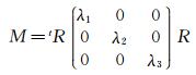
where R is the matrix of the eigenvectors of the Hessian ,and the λi are defined by:
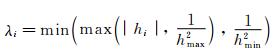
with hmin (respectively hmax) the minimum (respectively maximum) size wanted for the mesh and hi the eigenvalues of Hu. Thus,in area of large physical variations,small elements are inserted,and in area where the solution is quasi constant,large elements are placed.
2 Numerical SchemesOur numerical simulations are performed on unstructured anisotropic meshes (2D-triangles and 3D-tetrahedra). The system of equations is discretized using residual distribution schemes [8, 10]. Those numerical schemes allow constructing a high order method with compact stencil to ease parallelism.
2.1 Residual Distribution Scheme ConstructionThe scheme that is used to solve the equations introduced in section 1.2 is a residual distribution scheme (RDS). Here is briefly explained how such schemes are built. More details can be found in [6].
Considering a 2D steady conservation equation:

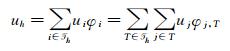
A tesselation Th of Ω is considered. Elements are noted T (boundary ∂T). Let uh=Σiuiφi,φi being the basis functions chosen on the triangle T. Eq. (9) integrated over Ω can be written as:
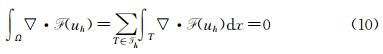
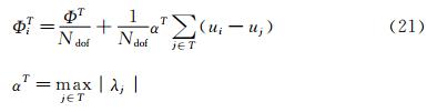
What is called the total residual ΦT can then be defined for each triangle:
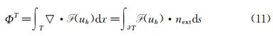
where next is the outward normal of the edges. The principle of a RDS is to distribute this residual to each degree of freedom (DoF) of the triangle (see Fig. 3). Each DoF receives what is called a nodal residual ΦiT using a coefficient distribution βiT

 |
| Fig. 3 Principle of a residual distribution scheme. Left: distribution for a P1 triangle; Right: gathering all triangles contributions. |
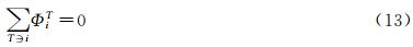
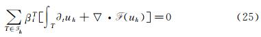
The distribution coefficients are defined according to the scheme used (Lax-Wendroff,Lax-Friedrichs,etc…). Then,all the contributions of each triangle where i belongs to are added (see Fig. 3),and the RDS is formulated as:
The solution of (13) can be obtained by solving the pseudo iterative scheme [5]:
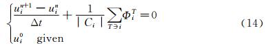
or more sophisticated iterative methods. An extension to the NS equations is defined in [7] and leads to an Eq. (13),with a total residual taking into account the viscous terms.
A RDS has a consistency property,is a positive scheme and is said linearity preserving.
Consistency: The distribution coefficients must satisfy
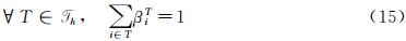
Nodal Residual Formulation: The nodal residual can be written as
Positivity: A positive RDS is a RDS with coefficient cijT defines such that

Positivity can be assimilated to the Total Variation Diminishing principle known for high order schemes. It ensures that no spurious oscillation appears.
Linear Preservation: A RDS is said linearity preserving if its distribution coefficients βiT are bounded

Two examples of RDS are described in the two next sections.
2.2 A Variant of the SUPG Scheme or Lax-Wendroff RDSAs said before,the RDS depends on the coefficient distribution chosen. The total residual is equally distributed to the DoFs and a stabilization term is added [7]. For P1 triangles,we have
The stabilization is defined such that both advection and diffusion are considered:
Looking at the Eq. (6),A is the Jacobian matrix of the advection: A=▽uF and K is such that: G=K▽U.
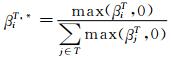
2.3 A Lax-Friedrich SchemeThe Jacobian matrix A is decomposed such as A=LΛR, where Λ=diag(λi) is a diagonal matrix and R,L are the matrices of the Eigenvectors. The nodal residual is written as:
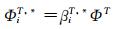
Then the distribution coefficient are defined by βiT=ΦiT/ΦT,but they can be unbounded (violation of the linearity preservation). Thus,a limitation is applied:
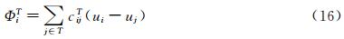
and the nodal residual is computed as follows
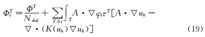
As for the previous scheme,this scheme is centered and needs a streamline dissipation term in smooth regions of the flow,the scheme is then given by
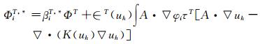
where τT is defined by Eq. (20),and ∈T(uh)≈1 in smooth regions and 0 close to discontinuities.
2.4 Validations on Numerical Test CasesUsing some test cases we demonstrate the ability of the proposed method to obtain an accurate solution along with an accurate wall treatment even when the initial mesh does not contain any point on the level-set 0.
2.4.1 Supersonic Flow Around a TriangleIn the first example we consider the supersonic flow around a solid body of triangular shape (height h=0.5,half angle θ=20°,see Fig. 4). The same computational domain as [11] is chosen and the computation is stopped when a steady state is obtained. The Lax-Friedrich RDS scheme is used for this numerical test case.
 |
| Fig. 4 Studied triangle and domain. |
Our initial mesh is only slightly adapted to the 0 level set (see Fig. 5(a)). The penalized variables are the velocity (uS=0) and the temperature (TS=3).
 |
| Fig. 5 Supersonic triangle test case. |
The Reynolds number is fixed to Re = 50 000 and the Mach number is chosen equal to Ma = 2.37 to get a shock in contact with the triangle peak.
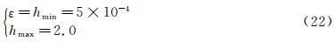
The component u of the velocity on the initial mesh is given in Fig. 5(b). For the adaptations,the following parameters (for both the level-set and the u-velocity) have been chosen:
The mesh obtained after 6 cycles of adaptation and the computed u-velocity on this mesh are presented in Fig. 6. A way to validate this test case is to compute the angle between the shock and the horizontal axis because this angle can be analytically computed. As in [1],the angle is measured using a point located on the shock at y=0 and we found β=53.33° for a analytic one of β ≈53.46°. As in Boiron et al. [11] an oblique shock is predicted and attached to the triangle,see Fig. 5(b) and Fig. 6. Our results are in good agreement with the theory and the numerical solutions performed in [11].
 |
| Fig. 6 Supersonic triangle,adapted mesh with the component u of the velocity isoline. |
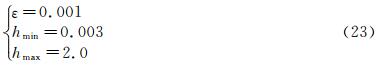
In this 3D test case taken from [1],the flow around an ellipse (sizes: (0.5,0.1,0.2)) centered in a spherical (radius r=10) domain is studied. The SUPG like RDS scheme is used for this numerical test. The parameters are set to Re=500 and Ma=0.375. As for the previous test case,the initial mesh is only adapted to the 0 level set (see Fig. 7(a)). The component u of the velocity obtained on this mesh is presented in Fig. 7(b). Two cycles of adaptation have been done with the following parameters (for both the level-set and the u-velocity adaptation):
 |
| Fig. 7 Flow around an ellipse. |
The adapted mesh is presented in Fig. 8(a),and its solution,the component u of the velocity in Fig. 8(b).
 |
| Fig. 8 Flow around an ellipse. |
Now we seek approximations of the solution of a time dependent problem defined by

Following a Petrov-Galerkin finite element approximation with
we ended up with,for any degree of freedom i,
Let mij being the mass matrix coefficient,we define the total flux of Eq. (24) by
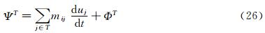
with ΦT defined by Eq. (11). The discrete counterparts of this equation are then given by
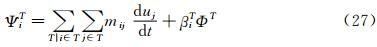
We propose to use the idea that in every T∈ Th the combination of terms arising from the multiplication of the mass matrix with the nodal time derivatives should give back an integral of the time derivative of uh over a dual sub-element cj∈T.
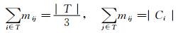
with |Cj|=βj|T| to guarantee the consistency.
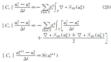
Following this idea the two steps of the explicit Runge-Kutta 2 (RK2) scheme are defined as follows
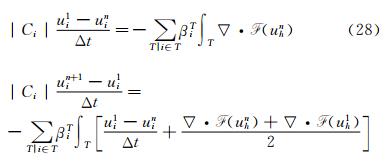
This construction of the explicit approach is based on three main points: first recast the RD discretization as a stabilized Galerkin scheme,then use a shifted time discretization in the stabilization operator,and lastly apply high order mass lumping on the Galerkin component of the discretization. All the details of the scheme and proofs can be found in [10].
3.1.1 Splitting ApproachThe accuracy of the penalization method depends on the value of η,in all steady simulations,we use an implicit scheme with η=1×10-12. For unsteady simulations the RK2 scheme described above is an explicit scheme. To overcome CFL restriction due to the penalty source term we propose a splitting algorithm. We solve step 1 and step 2 of Eq. (28) for the classical Navier-Stokes equations,without the penalty source term,then we add a third step to take into account implicitly the penalty source term.
3.1.2 Numerical Test on an Oscillating and Pitching Airfoil
In this test case,we model an oscillating wing experiencing simultaneous pitching θ(t) and heaving h(t) motions. The infinitely long wing is based on a NACA 0015 airfoil.
The pitching axis is located along the airfoil chord at the position (xp,yp)=(1/3,0). The airfoil motion is defined by the heaving h(t) and the pitching angle θ(t) defined as follows
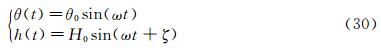
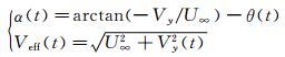
where H0 is the heaving amplitude and θ0 is the pitching amplitude. The angular frequency is defined by ω=2πf and the phase difference ζ is set to 90°. The heaving velocity is then given by

Based on the imposed motion and on the upstream flow conditions,the airfoil experiences an effective angle of attack α(t) and an effective upstream velocity Veff(t) defined by
An operating regime corresponding to the parameters Re=5 000,H0/c=0.5,f=0.14 and θ0=40.1deg has been computed.
Fig. 9 shows preliminary results for the vorticity at four different times on the fixed unstructured mesh. The motion of the wing is imposed using Eqs. (30) and (31) thanks to the penalty source term. Snapshot of the u-component and v-component of the velocity at time t=2.72 are presented in Fig. 10 showing that the penalized components of the velocity are not constant through the wing.
 |
| Fig. 9 Zoom of the NACA 0012 oscillating and pitching airfoil mesh along with vorticity contours. |
 |
| Fig. 10 Wind turbine test case,snapshot at time t=2.72. |
For this test case the interface of the NACA airfoil is moved at each time step and the sign distance function is computed for each new position as described in section 1.1.
3.2 Investigation on Unsteady Mesh AdaptationFurther investigations are performed to deal with moving bodies. The first step consists in following the moving body with the adapted grid. Two different approaches can be studied,the first one consists in solving the advection equation which governs the level-set evolution and the second one computes the whole signed distance function on the mesh after each displacement as it has been done in the previous test case.
For the first approach,as the body is defined by the sign distance function φ,for a body moving at speed V(t,x),the SDF is then governed by the following advection equation
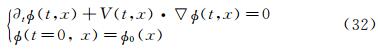
where φ0(x) corresponds to the initial position of the object,i.e the initial SDF. Here again the goal is to adapt the mesh to zero isoline of the level-set,and this time at each time step. As studied in [4],a characteristic method can be used. The nodes at time tn+1 are considered and their “original position” at time tn is searched by tracing back the characteristic. The mesh is then adapted to this new SDF. As we want to deal with physical displacements,time steps are very small and so are the displacements. Instead of using an iterative process as presented in [4],due to the small movement,the new zero level-set is defined in an already adapted area. Indeed as explained in section 1.3,when adaptation to zero level-set is done,the vicinity W of the zero level-set is also refined. Then,just after the advection,adaptation can be done.
A well known problem when dealing with level-set advection is the mass loss. Indeed,each advection leads to a small deformation of the surface. Therefore,another way of thinking is,instead of advecting the whole signed distance function,only the surface defining the solid is advected,and the SDF is computed using the method presented in section 1.1. This is the second approach. With this second approach,no mass loss is introduced. The problem is that computational time for large meshes is considerably higher than with the advective method. Consequently,our idea is to find a way of coupling advection and SDF computation to choose the best compromise between CPU time and quality of the solution.
4 ConclusionsIn this work,we combined the simplicity given by the penalization method to compute flow solutions around complex geometries with the power of mesh adaptation to improve accuracy. The accuracy is seek in the localization of the 0 level-set function (to be able to impose correctly boundary conditions inside our IBM) and also in the physical solution (to correctly capture shock waves for example). Another advantage of using IBM is the facility of studying moving bodies. To be able to perform unsteady computations we are studying a way of tracking interfaces on a mesh.
The idea is to advect during (N-1) time steps the SDF,and every N time steps to advect the surface to compute the whole SDF (see Fig. 11).Fig. 12 presents the displacement (rotation + translation) of a 3D quadrangle([-0.1,0.1]×[-0.2,0.2]×[-0.05,0.05]) and Fig. 13 shows a 2D oscillating and pitching NACA airfoil. The next step will be to couple this unsteady mesh adaptation process to our unsteady penalized residual distribution schemes.
 |
| Fig. 11 Adaptation process,Ti,Soli and Surfi denote respectively mesh,solution and surface at time i. |
 |
| Fig. 12 Moving quadrangle,top: isosurface; bottom: mesh cut with level-set. |
 |
| Fig. 13 Oscillating NACA airfoil. |
Acknowledgement:
● Experiments presented in this paper were carried out using the PlaFRIM experimental testbed,being developed under the INRIA PlaFRIM development action with support from LABRI and IMB and other entities: Conseil Regional d′Aquitaine,FeDER,Bordeaux University and CNRS (see https://plafrim.bordeaux.inria.fr/).
● Computer time for this study was provided by the computing facilities MCIA (Mesocentre de Calcul Intensif Aquitain) Université de Bordeaux et Universitéé de Pau et des Pays de l′Adour.
● This study has been carried out in the frame of the investments for the future,Programme IdEx Bordeaux,CPU (ANR-10-IDEX-03-02).
● R. Abgrall was supported by part by SNFS grant #200021_153604/1.
| [1] | Abgrall R,Beaugendre H,Dobrzynski C. An immersed boundary method using unstructured anisotropic mesh adaptation combined with level-sets and penalization techniques[J]. JCP,2014,257: 2014,83-101. |
| [2] | Dobrzynski C ,Frey P. Anisotropic delaunay mesh adaptation for unsteady simulations[C]//Proceedings of 17th Int. Meshing Roundtable,Pittsburgh,USA,2008. |
| [3] | Frey P,Alauzet F. Anisotropic mesh adaptation for CFD computations[J]. Comput. Methods Appl. Mesh. Engrg.,2005,194:5068-5082. |
| [4] | Dapogny C. Bui C,Frey P. An accurate anisotropic adaptation method for solving the level set advection equation[J]. Int. J. Numer. Meth. Fluid,2011. |
| [5] | Abgrall R,Roe P L. High order fluctuation schemes on triangular meshes[J]. J. Sc. Comp.,2003,13: 1-3. |
| [6] | Abgrall R. Essentially non-oscillatory residual distribution schemes for hyperbolic problems[J]. J. Comput. Phys.,2006,214(2): 773-808. |
| [7] | Abgrall R,De Santis D. High order residual distribution scheme for Advection-Diffusion problems[J]. Siam J. Sci. Comput.,accepted,2014. |
| [8] | Abgrall R,Larat A,Ricchiuto M. Construction of very high order residual distribution schemes for steady inviscid flow problems on hybrid unstructured meshes[J]. JCP,2011,230(11):4103-4136. |
| [9] | Dapogny C,Frey P. Computation of the signed distance function to a discrete contour on adapted triangulation[J]. Calcolo,2012,49:193-219. |
| [10] | Ricchiuto M,Abgrall R. Explicit Runge-Kutta residual distribution schemes for time dependent problems: second order case[J]. JCP,2010,229(16): 5653-5691. |
| [11] | Boiron O,Chiavassa G,Donat R. A high-resolution penalization method for large Mach number flows in the presence of obstacles. Computers and Fluids,2009,38(3):703-714. |