


2. 英国爱丁堡大学工学院, 爱丁堡 EH9 3JL
2. School of Engineering, The University of Edinburgh, United Kingdom, EH9 3JL
0 Introduction
The NS equations proposed in 1845 are very difficult to solve in their complete form. It’s always the goal of viscous fluid dynamics to search a simplified and accuracy enough solution for NS equations. In 1904,Prandtl proposed boundary layer theory which provided such a decisive simplification of the NS equations and opened up a new area of fluid dynamics[1]. From 1930’s to the 1960’s,various special second-order corrections[2, 3],interacting boundary layers[4] and higher-order boundary-layer theory[5] was developed in order to take viscous/inviscid interacting into consideration. From 1960’s,numerous authors from America[6, 7, 8],Russia[9],China[10] nearly contemporaneously independently developed and used some other approximate equations for solving viscous flow problems which are nearly boundary-layer type,but due to the physics of the problem being considered,include some additional effects either in the boundary conditions or the equations themselves. These different approximate equations with different slightly viscous terms have often been called “parabolized”,“thin layer”,“reduced” NS equations or “ISF” equations for obvious reasons. In the paper we simply call these classes of equations as PNS equations although it is somewhat a misnomer,since the equations are actually a mixed set of hyperbolic parabolic elliptical equations,provided that certain conditions are met.
Amounts of numerical simulation shown that solution of PNS equations were closed to solution of full NS equation for flows without large separation. Also,for high Re number flows,if the solution of full NS equation were taken based on a set of coarse mesh,because of real physical viscous being covered by numerical viscous,the final solution are not numerical result of full NS equation but numerical result of another set of reduced NS equations,such as PNS equations[11]. On the other hand,because strong viscous region only is existing in shear layer and region near the wall surface and most of the rest region were dominated by non-viscid flows,simple PNS equations will be enough to describe high Re viscous flows instead of full NS equations [12].
A set of PNS equations is of theoretical value in establishing Prandtl’s approximation as the basis of an asympototic solution of the NS equations for large Re number. It may also be of practical value. “The PNS method is in very wider spread use; indeed,it forms the basis of an industry-standard computer program,which is used by virtually all major aerodynamic laboratories and companies.” as Anderson pointed in his monograph[13]. Furthermore,the development of such a technique requires the examination of the fundamental (asymptotic) structure of the flowfield which leads not only to the determination of the correct approximate equations to use but also to the scale laws which set the mesh sizes for accurate numerical computations. This information is necessary even if one wishes to efficiently solve the full NS equations.
For a significant class of asymptotic approximations to the complete NS equations,PNS equations would have correctly accounted for viscous-inviscid flow interacting mechanism and opened a new approach for simulating large Re number flows[14]. The present paper addresses the basis and advantages of various different PNS equations with different slightly viscous terms and different name,including viscous/inviscid interacting shear flow (ISF) theory proposed by professor Gao in the late 1960s,which can be regarded as a type of PNS’s basic theory. Several inferences of ISF theory and their applications to computational fluid dynamics (CFD) are also discussed in the paper.
The present paper is organized as follows. A briefreview of different PNS equations and their mathematical properties,numerical solution method are given in section 1. A kind of PNS equations,ISF theory,proposed independently by Chinese author is presented in section 2. Section 3 will show that some inferences of ISF theory such as wall-surface criteria formulas and new pressure boundary conditions derived from ISF equations also have important value to CFD application. Some conclusions are finally drawn in section 4. 1 A brief review of PNS equations 1.1 Different form and mathematical properties of PNS equations
The derivation of PNS equations from the complete Navier-Stokes equations is,in general,not as rigorous as the derivation of the boundary-layer equations. Because of this,slightly different versions of the PNS equations have appeared in the literature. These versions differ in some cases because of the type of flow problem being considered. However,in all cases the normal pressure gradient term is retained,and the second derivative terms with respect to the streamwise direction are omitted.
As Pletcher classified[15],there are several sets of equations that fall within this class,such as parabolized Navier-Stokes (PNS) equations[8, 16],reduced Navier-Stokes (RNS) equations,partially parabolized Navier-Stokes (PPNS) equations,viscous shock-layer (VSL) equations,conical Navier-Stokes (CNS) equations,and thin-layer Navier-Stokes (TLNS) equations. The most common form of PNS equations[17] is obtained by assuming that the streamwise viscous derivative terms are of O(1),while the normal and transverse viscous derivative terms are of O(ReL1/2). Hence these PNS equations are derived by simply dropping all viscous terms containing partial derivatives with respect to the streamwise direction from the steady NS equations.The PNS equations in generalized coordinates[18] can also be obtained by simply dropping the viscous terms containing partial derivatives with respect to the streamwise direction ξ.
For simplicity,let us consider the 2-D PNS equations and assume a perfect gas with constant viscosity to examine the mathematical nature of the PNS equations.
Where

Note that in these equations a parameter ω has been inserted in front of the streamwise pressure gradient term in the x momentum equation. Thus if ω is set equal to zero,the streamwise pressure gradient term is omitted. On the other hand,if ω is set equal to 1,the term is retained completely.
The mathematical property of PNS equations had been studied by many authors. Detail characteristic analysis procedure can be found in literatures[19, 15]. If the streamwise pressure gradient is retained completely(i.e., ω =1),only when local streamwise Mach number Mx>1 an initial-boundary value hypothesis of PNS equations is well-posed,i.e. PNS equations can be solved numerically by space marching algorithm(SMA) along the x-direction,while when Mx<1,an initial-boundary value hypothesis is ill-posed. But if only a fraction of the streamwise pressure gradient is retained (i.e.,0≤ ω <1),PNS equations can be solved by SMA when  When we need to retain the streamwise pressure gradient term fully in the subsonic portion of the boundary layer,since an “elliptic-like” behaviour is introduced. A number of different techniques have been proposed to circumvent this difficulty[20, 15].
There is a novel technique for handling the streamwise pressure gradient term using the concept of splitting the term into its “elliptic” and “hyperbolic” components. This has led to the introduction of a new set of equations called the RNS equations[21]. The RNS equations are derived from the complete unsteady Navier-Stokes equations by dropping the streamwise viscous terms,omitting the viscous terms in the normal momentum equation,and splitting the streamwise pressure gradient using 
 In most applications,the time-derivative terms are also omitted.

 which represents “elliptic” components of the pressure gradient term.
For supersonic flows with embedded “elliptic” regions,the global pressure relaxation procedure can be used to solve the RNS equations. For subsonic flows,if PNS equations are solved without making simplifying approximations regarding the pressure,the equations are only partially parabolized,leading to the terminology PPNS.
The PPNS system remains elliptic overall because of the influence of the pressure field.In developing the PPNS model from the Navier Stokes equations,only certain diffusion processes are neglected,and no assumptions are made about the pressure. The PPNS model has also been referred to as the semi-elliptic or RNS formulation in the literature. PPNS may be regarded as a specified name of PNS for subsonic flows. The solution strategies employed for the PPNS model can be distinguished as either pressure-correction schemes[22] or coupled approaches[23]. Multiple streamwise sweeps are required in both approaches.
The VSL equations are a more approximate set of equations than the PNS equations,such as used by Davis[24]. In 2-D Cartesian coordinates,the continuity and x momentum equations are the same for VSL and PNS but the y momentum and energy equations in the VSL set of equations are simpler than the corresponding PNS equations.
CNS equations were referred to the equations solved subject to a local conical approximation,which was firstly suggested that a quick estimate of the heat transfer and skin friction could be obtained by solving the unsteady NS equations on the unit sphere with all derivatives in the radial direction set equal to zero byAnderson[15].
The thin-layer Navier-Stokes equations were obtained upon simplifying the complete NS equations using the thin-layer approximation which was arisen from a detailed examination of typical high Re number computations involving the full NS equation by Baldwin and Lomax[25]. Thin-layer approximation can also be used into PNS equations. The typical resulting TNLS equations can be seen in many literatures[26, 27]. The TLNS equations are a mixed set of hyperbolic-parabolic PDEs in time.
All kinds of PNS equations can extend to turbulent flows using similar approximation to obtain simplified parabolized Reynolds Averages Naiver-Stokes (PRANS) equations. 1.2 Numerical solution of PNS equations
PNS computational techniques are the most key of PNS and also basic reason of PNS becomes the basis of industry-standard aerodynamic computations. For the PNS system,streamwise ξ diffusion terms are neglected,or with other higher order diffusion terms are treated as an explicit deferred corrector. This formulation reduces to a single sweep or initial value PNS method,whenever the negative flux contributions due to acoustic and convective upstream influence can be uniformly neglected. This proceduce is very computer efficient. If the negative flux terms are important and retained,an alternative formulation to conventional characteristic-based flux differencing results. This procedure is applicable for incompressible to hypersonic flows and allows for upstream influences due to strong shock interactions and confined regions of reverse flow. Relaxation procedures (in ξ) with multigrid acceleration have proven very effective for subsonic and supersonic interacting flows. For incompressible flows,artificial compressibility or Poisson pressure solvers are not required. For supersonic flows with moderate interaction,global relaxation or multiple-sweep PNS methodology is effective. For strong interactions,sharp shock and revers flow capturing,without added numerical viscosity,is possible with relaxation,sparse matrix direct solvers,or other factorizations. The detail overview of PNS computational techniques can be found in literatures[18, 20].
In recent years,PNS algorithms were focus on how to increase convergence speed and how to deal with large reverse-flow regions or subsonic-flow regions,and their extending to non/structure grids. One method is using a space-marching scheme solving the PNS equations until an elliptic/reverse-flow region is encountered,then switching to a global iteration method for the length of the elliptic region,iterating until convergence is reached,and pursuing with the marching PNS scheme. However,such a strategy forces the solution of the PNS equations in certain regions of the flow field,for which the PNS assumption might induce appreciable errors. The accuracy of the final solution is hence strongly dependent on the ability of the method to predict correctly different flow regions. Another approach,named “active domain,” to solving inviscid supersonic flow with embedded subsonic regions has been proposed. The method consists of performing pseudo-time iterations on a small bandlike computational domain that advances in the streamwise direction every time the residual of the active domain near the upstream boundary falls below a user-defined threshold. Using sensors based on the streamwise components of the Mach number,the active-domain boundaries automatically surround any locally subsonic region on which sufficient iterations are performed to reach steady state. When the residual inside the subsonic region decreases below the user-defined threshold,the active domain advances past the subsonic region further downstream. By marching in the streamwise direction,the active domain results in up to a 10-fold decrease in work compared to standard pseudo-time-marching methods for several inviscid problems. However,the ability of the active domain to solve accurately a streamwise elliptic region is limited by the accuracy of the sensor responsible for the upstream movement of the upstream boundary of the active domain. Extension of the active-domain method to viscous flow is hampered by the difficulty of formulating a streamwise ellipticity sensor that captures all significant upstream propagating waves while restricting the size of the active domain to a minimum. In 2002,Parent et al.[28] extended the active-domain method to streamwise separated flows. An alternate form of the active-domain method,named the “marchingwindow” algorithm which was applicable to streamwise separated flows was developed. The marching window performs localized pseudo-time stepping on a sub-domain composed of a sequence of cross-stream planes of nodes. The width of the marching window decreases to only a few planes in regions of quasihyperbolic flow and increases to the size of the streamwise-elliptic region when encountered. However,the marching window is strictly a convergence acceleration technique,as it guarantees that the residual of all nodes will be below the user-defined threshold when convergence is attained. This is accomplished by keeping the residual upstream of the marching-window sub-domain updated at all times,and by positioning the upstream boundary such that the residual of all nodes upstream is below the user-defined threshold. This results in an algorithm that captures all upstream propagating waves affecting the residual significantly. The upstream propagating waves can originate from (but are not necessarily limited to) large subsonic pockets,streamwise separation,streamwise viscous fluxes,or flux limiters in the streamwise convection flux derivative,for instance. 1.3 Applications of PNS and its’ fluid theory
The PNS method has been widely utilized in virtually all major aerodynamic laboratories and companies for many cases including perfect gas flows,chemically reaction flows[29],and magneto-hydrodynamic(MHD) flow[30],etc. There are several (more than ten) space marching PNS special softwares,such as AFWAL PNS[31],NASA UPS[32],IMPNS[33],TORPEDO[34] and SSPNS[35],codes by He[36]. Many research about PNS method are focus on the instability,speed,efficiency,application scope of space marching algorithm but few literatures talk about fluid basic theory of PNS.
As we have known that the boundary layer (BL) theory reveals a basic flow: viscous thin layer without interaction between it and outer inviscid flow. Based on this basic boundary layer theory BL equations were derived and many excellent and important theory results,such as zero normal pressure gradient,were given,besides of marching algorithm for BL equations.
However,it is not very clear what kind of basic flow is described by the PNS equations before the 1990s,there is also no basic fluid theory corresponding PNS equations. The monograph[15] published in 1997 introduced PNS still in this manner: they are suitable to several typical flows,such as (a) Leading edge of a flat plate in a hypersonic rarefied flow. (b) Mixing layer with a strong transverse pressure gradient. (c) Blunt body in a supersonic flow at high altitude. (d) Flow along a streamwise corner (e) Flow in rectangular channals. Stagnation point flow or oblique incidence stagnation point flow and multi-layer (Triple-deck) flow with its outside inviscid flow have also been proved applicable to PNS theory.
A PNS’s basic fluid theory,viscous/inviscid interacting shear flow (ISF) theory,was suggested by Gao[37] and it may furnishes complete answer to the subject in last paragraph. ISF consists of viscous shear flow and its neighboring outer inviscid flow,which interact on each other. The equations governing ISF are just kind of PNS equations. ISF theory forms basic fluid theory for PNS equations and it also makes a breakthrough the beyond the classical boundary layer theory. Furthermore,some novel inferences were derived based on ISF theory and they have some important applications to CFD,such as application of ISF’s optimal coordinates to grid design,application of length scaling laws of ISF’s viscous layer to grid design,using small scale structure given by the scaling-laws to explain and capture sudden changes of physical quantities like pressure of heat flux on body surface which are called “unknown-unknown” for hypersonic flow by Bertin and Cumming[38],application of wall-surface-criteria for laminar flow,perturbed flow and turbulent flow to verify creditabilities of NS and RANS numerical solutions and to optimize turbulent models etc. 2 ISF theory and its i nferences
The motion-law,maybe the core hypothesis,of ISF’s viscous layer is convection-diffusion competitive in its normal direction,while it is convection-dominant in its streamwise direction. For simplicity,the mathematical definition formula of this motion-law can be expressed as following[39]:
Where the x and y are coordinate variables of a fitted dividing-flow-surface orthogonal coordinates,that is called ISF’s optimal coordinates,otherwise the definition formula (3) and (4) does not hold. There is always a dividing-flow-surface in ISF’s viscous layer [40],especially,the wall surface is a dividing-flow-surface of viscous flow close neighbour wall surface. f=(u,v,T),u and v are velocity components in the x- and y- directions,respectively. T is the temperature,λ=ν if f=u and v,λ=k if f=T,ν is the kinematics viscous coefficient,k is the thermal conductivity.
Using the definition (3) and (4) to simplify complete NS equations,we can deduce the ISF equations,that is for two-dimension compressible flow

If we compare ISF equations with PNS equations introduced before,we’ll find that they are in the same forms. It implied that ISF equations are one type of PNS equations. But different from PNS equations,ISF equations go further more in theory analysis and deduced many useful inferences,just like boundary layer theory generate much more excellent theory results. 2.1 Inference 1: The evolution physical scales of ISF’s viscous layer
Scaling-laws of velocity and length of ISF’s viscous layer were examined by Gao[41]. The physical scales of 3-D incompressible flow can be expresses generally as:
(xp,yp,zp;up,vp,wp)=
Where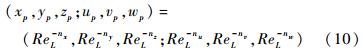
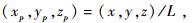
 supposing the reference length of ISF is L,reference velocity is U. It is assumed and had been proved correct that kinetic energy dissipation in ISF’s viscous layer is independent of ReL. Using the hypothesis and equations (3)-(9),we can deduce
Where q=ln
supposing the reference length of ISF is L,reference velocity is U. It is assumed and had been proved correct that kinetic energy dissipation in ISF’s viscous layer is independent of ReL. Using the hypothesis and equations (3)-(9),we can deduce
Where q=ln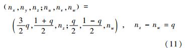
 /ln ReL,which is called interaction parameter and has been proved that 0≤q≤1/2. If w can be compared with u,when q=0 ISF expresses the stagnation flow or the classical boundary-layer flow and its neighbouring outer in-viscid flow,between which there is no interaction; when q=1/4 the ISF’s viscous layer is just the lower deck of the well-known triple-deck theory[41],in this case ISF express flow in neighbourhood of separation point or reattachment point or tail-edge point or leading edge point or small step,hump,dents and chinks on wall surface etc. when q=1/2 the length scales and velocity scales of ISF’s viscous layer are the same in all directions,i.e. an isotropic viscous flow. Therefore,the interacting parameter q is essentially a measure of strength of viscous/inviscid interaction. In addition,if the effects of the Mach number or say compressibility are not neglected,we can deduce further the scaling-laws of the density and temperature,adding which to know scaling-laws. It should be pointed out that the evolution laws of physical scales (10) also suitable to free ISF,for which there is less study.
ISF can express some typical flows mentioned above. The whole viscous/inviscid interacting flow in the neighbourhood of wall surface is obviously a complex ISF,whose governing equations are diffusion parabolized equations written in a fitted body orthogonal coordinates,which is just a fitted dividing flow surface orthogonal coordinates or say the complex ISF’s optimal coordinates. 2.2 Inference 2: Dividing flow surface criteria
In ISF’s viscous shear layer there is always a dividing flow surface with normal velocity v=0 in ISF’s optimal coordinates,such as the mixed layer flow,the jet and flow between circular-flow and outer inviscid flow of a separation flow etc. The ISF equations can be simplified further on the dividing flow surface and the resultant equations are called dividing flow surface criteria[42, 43],that is for a 2-D compressible flow
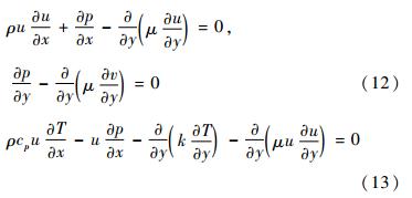
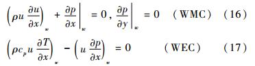
Two important special cases of dividing flow surface criteria (12) and (13) are wall-surface criteria (WSC) for viscous flow and inviscid flow near the wall. This two WSC are respectively
And where WMC and WEC are wall momentum criteria and wall energy criteria,respectively. They can be used to verify creditability of numerical simulations for viscous flow or inviscid flow near wall surface.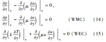
It should be pointed that ISF theory and its inferences can also be extended into perturbed flow and turbulent flow. Both interacting shear perturbed flow (ISPE) theory and interacting shear turbulent flow (ISTF) theory were also suggested by Gao[44]. As space is limited,ISPE,ISTF and their inferences can be referenced in literatures [45]. In order to uniform the name,ISPE can also be called parobolized stability equation (PSE). ISTF can be called parabolized Reynolds average NS (PRANS). Both PSE,PRANS equations and their theories,that are closely related PNS and its theory,will be review in future. 3 Some applications of ISF theory in CFD[46] 3.1 Application of ISF’s small-scale-structure concept
The scaling laws of ISF’s viscous layer reveal that small-scale structure generate certainly in ISF’s viscous layer flow,that will do induce sudden changes of several physical quantities like wall heat flux and pressure gradient etc and its gradient. As an example,for the case of laminar ISF and Re=106,temperature gradient in local interaction zone increase 5.7 times in normal direction and 31.6 times in flow direction than before interaction(q=0) if q=1/4.
It is known that to date there no very convincing numerical results of using ISF’s scaling laws to compute sudden increase of local heating rates etc. However,we ought to pay highly attention to thus computations for sudden change phenomena. This is because that some flight accidents,such as the damage of the rocket-powered X-15 when its flight velocity reached Mach 6.7 in 1967 and the demise of the space shuttle Columbia during its re-entry from orbit in 2003. These accidents show that how severe the aero-thermodynamic environment is for a vehicle which is travelling at hypersonic speeds and that how fragile the vehicles that fly through these environments can be. Analysis about mentioned above flight accidents making Bertin and Cummings[38] giving the following conclusions: “These locally severe,critical heating rates or unexpected deviations to the force and moments acting on the vehicle often occur due to viscous/inviscid interactions. These critical environments are the result of ‘unknown-unknown’ or ‘gotchas’ ”.
In fact,the scaling-laws of ISF’s viscous layer have illustrated the mechanism of the sudden change phenomena of heating rates etc. and offered a way to compute locally sudden change or at least a roughly order of magnitude estimate of them. 3.2 Application of optimal ISF’s coordinates to guide grid design
For computations of ISF and flow near wall surface,an optimal grid should be an orthogonal grid with grid-line paralleling with the coordinate axes of ISF’s optimal coordinates. One example is to compute two-dimensional incompressible mixing layer flow [47],refer to Fig. 1-4. Two grid systems are used,one is an optimal orthogonal grid the other is the resultants of the optimal grid rotating anticlockwise 45°. The maximum gradients of velocity and temperature given by the latter are respectively about 40% and 50% of those given by the former grid. Thus errors influence the transit of momentum and energy across ISF’s viscous layer and also affect the flow in downstream.
 |
| Fig. 1 Two dimensional mixing flow |
 |
| Fig. 2 Optimal and non-optimal grid sketchs |
 |
| Fig. 3 Velocity profile with different grids |
 |
| Fig. 4 Temperature profile with different grids |
Therefore,in order to compute exactly various ISF occurring in flow field computed,we ought to use ISF’s optimal grid each individual,such as a base free ISF between base circulatory flow and outer inviscid flow and a complex free ISF between circulatory flow in separation region and outer inviscid flow and a complex viscous/inviscid interacting flow in the neighbourhood of wall surface. Obviously,the three ISF’s optimal orthogonal grids are completely different. For the complex ISF in the neighbourhood of wall surface,the complex ISF’s optimal coordinates are just fitted body orthogonal coordinates,having to use which in computing flow over a body is well-known to all. 3.3 Application of the length scaling- laws of ISF’s viscous layer to determine appropriate mesh size
The grid size is responsible for accuracy of numerical simulations. For the direct numerical simulation of turbulent flows,Kolmogorov scale is an important reference scale to choosing grid size. For boundary layer flow,thickness of boundary layer maybe a reference length. However,for an ordinary computation of Navier-Stokes equations,there was no definite method or standard to choosing grid size in the past. Obviously,the length scaling-laws given by ISF’s theory would be a definite method to determine an appropriate mesh size,that have been proved tentatively by two sets of computation solving NS equations[48].
An analysis for the numerical results of hypersonic flows over both an asymptotic hollows cylinder extended flare(HCEF) and a sharp double cone(SDC) shows that in this two examples the better numerical solutions can be obtained(refer to Fig. 5-11) when the grid sizes in both streamwise and normal directions are directly chosen as 1/10 of the length scale with q=1/4 (see formula (10)and (11)),that can avoid refining repeatedly grid for seeking the best grid size. It should be emphasize on the importance of both ISF’s optimal coordinates and the length scaling-law of ISF’s viscous layer to grid design. Just as Schlichting and Gerstin pointed out in their monograph[40]: “Numerical methods in computing flows at high Reynolds numbers only become efficient if the particular layered structure of the flow,as given by the asymptotic theory,is taken into account,as occurs if a suitable grid is used for computation.”
 |
| Fig. 5 Computational domain and pressure contour |
 |
| Fig. 6 Pressure coefficient for HCEF,Run 8 |
 |
| Fig. 7 Stanton number for HCEF,Run 8 |
 |
| Fig. 8 Detail of Fig. 6 around separation point |
 |
| Fig. 9 Detail of Fig. 6 near attachment point |
 |
| Fig. 10 Pressure coefficient for Run 28 over SDC |
 |
| Fig. 11 Stanton number for Run 28 over SDC |
Obviously,ISF theory shows further that numerical computations of high Re number flow only become efficient if the thin-layered structure in all directions,given by ISF theory,is taken into account,as occur if a suitable grid with grid-lines paralleling the coordinate axes of ISF’s optimal coordinates and with grid-refined locally according to the length scale of the small-scale structure in ISF’s viscous layer is used for computations. 3.4 Application of the wall-surface criteria to verify creditability of NS numerical solutions
The existence and uniqueness of the solution of NS equations have not been proved. So we have to face to an always confused problem--is it worth to trust the results from computer codes? If it does,how much can we trust it? Verification and validation of computing results become a very important work. The dividing flow surface criteria and wall surface criteria (WSC) are undoubtedly theoretical methods of verifying creditability of NS numerical solution. Except for WEC,Gao[41] had confirmed that eleven well-known NS exact solutions for incompressible flow satisfy exactly WSC and that both the solution of the classical boundary layer and its outer inviscid flow and the solutions of similar boundary layer with its outer inviscid flow satisfy WSC and that the local solution of ISF with q=1/4 ,i.e. the solution of Triple-deck theory[43] satisfies WSC. Therefore,NS numerical solutions also ought to satisfy WSC,which are proved numerically by some computations of two-dimensional incompressible stagnation flow[49],shock/boundary layer interacting flow[50],compression ramp and cylinder flare[51],refer to Fig. 12-Fig. 15.
 |
| Fig. 12 WMC in shock laminar boundary layer interacting flow |
 |
| Fig. 13 WEC in shock laminar boundary layer interacting flow |
 |
| Fig. 14 WMC in laminar hypersonic flow over ramp |
 |
| Fig. 15 WEC in laminar hypersonic flow over ramp |
In a word,we can obtain NS grid independent solution by operation of NS numerical calculations satisfying progressively the wall surface criteria (WSC). Especially,this criteria can evaluate the departure of NS numerical solutions from NS true solution by just one time NS calculation on set of grid,which is an outstanding advantage of the WSC method compared with the grid convergence analysis method in common use,based on that some people[5, 15, 16, 17] suggested that the WSC method may be used as an ingenious substitute for the grid convergence analysis method and that the WSC method and ISF theory would be called Gao’s criteria and Gao’s ISF theory,respectively. 4 Conclusions
As a class of equations to describe fluid flows,PNS equations have been used to successfully compute the 3-D subsonic supersonic/hypersonic viscous flow over a variety of body shapes or internal viscous flows. Solving PNS equations forms industry-standard aerodynamic and aero- thermodynamic computations. The PNS method is in very widespread use. For PNS methods,attention should be paid not only on developing space marching algorithm but also on developing basic PNS theory.
The ISF theory offer a basic fluid theories corresponding to PNS. The ISF equations are one kind of PNS equations. Some inferences from ISF theory and their application to CFD are fruitful and creativeness. Scientific computation of aerodynamic and aerothermodynamic phenomena does need to integrate well computation with fluid theory,especially for hypersonic flow computation.
Acknowledgements:I am very thankful to Prof. Z. Gao for helpful discussion. Acknowledgement is also made to the support of China Scholarship Council and host of Professor Khellil Sefiane in School of Engineering,University of Edinburgh.
| [1] | Cebeci T, Cousteix J. Modeling and computations of boundary layer flows[M]. New York: Springer, 1999. |
| [2] | Van Dyke M. Higher approximations in boundary layer theory. Part 1: General analysis[J]. J. Fluid Mech., 1962, 14: 161-177. |
| [3] | Van Dyke M. Higher approximations in boundary layer theory. Part 2: Application to leading edges[J]. J. Fluid Mech., 1962, 14: 481-495. |
| [4] | Dechaume A, Cousteix J, Mauss J. An interactive boundary layer model compared to the triple deck theory[J]. Eur. J. Mech. B Fluids, 2005, 24(4): 439-447. |
| [5] | Van Dyke M. Higher-order boundary-layer theory[J]. Annu. Rev. Fluid Mech., 1969, 1: 265-292. |
| [6] | Davis R T, Flugge-Lotz I. Second-order boundary-layer effects in hypersonic flow past axisymmetric blunt bodies[J]. J. Fluid Mech., 1964, 20(4): 593-623. |
| [7] | Davis R T. Numerical solution of the hypersonic viscous shock-layer equation[J]. AIAA J., 1970, 8(5): 843-851. |
| [8] | Rudman S, Rubin S G. Hypersonic viscous flow over slender bodies with sharp leading edges[J]. AIAA J., 1968, 6(10): 1883-1889. |
| [9] | Golovachov Y P, Popov F D. Supersonic viscous flow past a blunt-body at high Reynolds numbers[J]. J. Computational Math And Mathematical Phys., 1972, 12(5): 1292-1303. (In Russian) |
| [10] | Gao Z. Simplified Navier-Stokes equations and simultaneous solution of viscous/inviscid boundary-layer[J]. Acta Mechanica Sinica, 1982, 14(6): 606-611. (In Chinese) |
| [11] | Zhang H X, Guo C, Zong W G. Problems about grid and high order schemes[J]. Acta Mechanica Sinica, 1999, 31(4): 398-405. (In Chinese) |
| [12] | Gao Z, Shen Y Q. Effects of physical and grid scales in difference computing of the Navier-Stokes equations[C]//Proc. of Inter. Conference on Applied Computational Fluid Dynamics, Beijing, China, October, 2000: 141-148. |
| [13] | Anderson J D Jr. Hypersonic and high temperature gas dynamics (2nd ed. )[M]. AIAA Education Series, 2006. |
| [14] | Zhuang F G, Zhang D L. Significance of diffusion-parabolized NS equations and its application to computational fluid dynamics[J]. Acta Aerodynamic Sinica, 2003, 21(1): 1-10. (In Chinese) |
| [15] | Tannehill J C, Anderson D A, Pletcher R H. Computational fluid mechanics and heat transfer(2nd ed.)[M]. New York, Hemisphere Press, 1997. |
| [16] | Cheng H K, Chen S Y, Mobley R, et al. The viscous hypersonic slender-body problem: a numerical approach based on a system of composite equations[R]. The Rand Corporation, 1970, RM-6193-PR, Santa Monica, California, . |
| [17] | Lubard S C, Helliwell W S. Calculation of the flow on a cone at high angle of attack[J]. AIAA J. 1974, 12: 965-975. |
| [18] | Rubin S G, Tannehill J C. Parabolized/reduced Navier-Stokes computational techniques[J]. Annu. Review Fluid Mech., 1992, 24: 117-139. |
| [19] | Gao Z. Hierarchial syructure of simplifying Navier-Stokes equations and mathematical property of simplified Navier-Stokes equations[J]. Acta Mechanica Sinca, 1988, 20(2): 107-116. (In Chinese) |
| [20] | Wang R Q, Shen Y Q. Numerical solutions of the diffusion parabolized Navier-Stokes equations[J]. Advance in Mechanics, 2005, 35(4): 481-497. |
| [21] | Rubin S G, Khosla P K. A review of reduced Navier-Stokes computations for compressible viscous flows[J]. J. Comput. Syst. Eng., 1990, 1: 549-562. |
| [22] | Pratap V S, Spalding D B. Fluid flow and heat transfer in three-dimensional duct flows[J]. Int. J. Heat Mass Transfer: 1183-1188. |
| [23] | Rubin S G, Lin A. Marching with the PNS equations[J]. Isr. J. Technol., 1981, 18: 21-31. |
| [24] | Davis R T. Numerical solution of the hypersonic viscous shock-layer equations[J]. AIAA J., 1970, 8: 843-851. |
| [25] | Baldwin B S, Lomax H. Thin-layer Navier-Stokes approximation and algebraic model for separated turbulent flows[R]. AIAA 1978-0257. |
| [26] | On implicit finite-difference simulations of three dimensional flow[R]. AIAA 1978-10. |
| [27] | Blottner F G. Significance of the thin-layer Navier-Stokes approximation, numerical and physical aspects of aerodynamic flows[M]. edited by Cebeci T., Springer-Verlag, New York: 1986: 184-205. |
| [28] | Parent B, Sislian J P. The use of domain decomposition in accelerating the convergence of quasihyperbolic systems[J]. J. Comput Phys., 2002, 179(1): 140-169. |
| [29] | Wadawadigi G, Tannehill J C, Buelow P E, et al. Three-dimensional upwind parabolized Navier-Stokes code for supersonic combustion flowfields[J]. J. Thermophysics and Heat Transfer, 1993, 7: 661-667. |
| [30] | Kato H, Tannehill J C, Gupta S, et al. Numerical simulation of 3-D supersonic viscous flow in an experimental MHD channel[R]. AIAA paper 2004-0317, 2004. |
| [31] | Shanks S P, Srinivasan G R, Nicolet W E. AFWAL parabolized Navier-Stokes code: formulation and user's manual[R]. AFWAL TR-82-3034, 1982. |
| [32] | Lawrence S L, Tannehill J C, Chaussee J C. An upwind algorithm for the parabolized Navier-Stokes equations[R]. AIAA 1986-1117. |
| [33] | Prince S A, Williams M J, Edwards J A. Application of a parabolized Navier-Stokes solver to some problems in hypersonic propulsion aerodynamics[R]. AIAA 2001-4066. |
| [34] | Moschetta J M, Lafon A, Deniau H. Numerical investigation of supersonic vertical flow about a missile body[J]. J. Spacecraft Rockets, 1995, 32: 765-770. |
| [35] | Chen B, Wang L, Xu X. An implicit upwind parabolized Navier-Stokes code for chemically nonequilibrium flows[J]. Acta Mechanica Sinica, 2013, 29(1): 36-47. |
| [36] | He X Z. Numerically simulate aero-froce&heat of hypersonic vehicles and region marching method for supersonic flow simulation[D]. [Ph.D Dissertation]. Mianyang: China Aerodynamics Research and Development Center, 2007. |
| [37] | Gao Z. Viscous/inviscid interacting shear flow theory[J]. Acta Mechanica Sinica, 1990, 22(1): 9-19. (In Chinese) |
| [38] | Bertin J J, Cummings R M. Critical hypersonic aerothermodynamics phenomena[J]. Annu. Rev. Fluid Mech., 2006, 38: 129-157. |
| [39] | Gao Z. Invariance of interactive-structure between convection and diffusion[J]. Acta Mechanics Sinica, 1992, 24(6): 661-670. |
| [40] | Schlichting H, Gersten K. Boundary-Layer Theory[M]. Springer-Verlag, Berlin, 2000. |
| [41] | Gao Z. Strong viscous layer flow theory with application to viscous flow computation[J]. Acta Aerodynamica Sinica, 2001, 19(4): 420-426. (In Chinese) |
| [42] | Gao Z. Interacting shear flow(ISF) theory, diffusion parabolized NS equations and wall-surface criteria and the applications[J]. Chinese Mechanics Abstracts, 2007, 21(3): 13-22. (In Chinese) |
| [43] | Gao Z. The wall-surface criteria with application to evaluate creditability of CFD simulation[J]. Acta Aerodynamica Sinica, 2008, 26(3): 378-393. (In Chinese). |
| [44] | Gao Z. The basis of an industry-standard aerodynamic computations and its theoretical basis with inferences and their application to CFD[J]. Procedia Engineering, 2013, 67: 230-240. |
| [45] | Gao Z, Shen Y Q, Zha G C. Viscous/inviscid Interacting shear flow theory with inferences and their applications to CFD[R]. AIAA 2004-1445. |
| [46] | Yu Y, Zhang H R. Gao's interacting shear flow (ISF) theory and its inferences and their applications[J]. Journal of Beijing Institute of Technology, 2013, 22(3): 291-300. |
| [47] | Yu Y. Mesh design of free shear layer flows simulation[J]. Transactions of Beijing Institute of Technology, 2013, 33(9): 885-895. (In Chinese) |
| [48] | Zhang H R, Yu Y. A guidance to grid size design for CFD numerical simulation of hypersonic flows[J]. Procedia Engineering, 2013, 67: 178-187. |
| [49] | Yu Y. New CFD validation method with application to verify computations of near wall flows[J]. Journal of Beijing Institute of Technology, 2010, 19(3): 259-263. |
| [50] | Hu J, Yang H, Yu Y. Wall-surface criteria and its application to verify computations of shock wave/laminar boundary layer[J]. Transactions of Beijing Institute of Technology, 2012, 32(8): 781-785. |
| [51] | Xu X W. Wall-surface criteria: a method of evaluating creditability of CFD, analysis and application[D]. [Master Degree thesis]. Beijing: Beijing Institute of Technology, 2012. (In Chinese) |