2. University of Chinese Academy of Sciences, Beijing 100049, China;
3. Key Laboratory of Time and Frequency Primary Standards, Chinese Academy of Sciences, Xi'an 710600, China
The Earth orientation parameters (EOP): universal time, xp, yp pole coordinates and nutation-precession corrections, describe the irregularities of the Earth′s rotation. Technically, they are the parameters which provide the rotation of the International Terrestrial Reference System (ITRS) to the International Celestial Reference System (ICRS) as a function of time. EOP derived from modern space geodetic technologies, e.g., Very Long Baseline Interferometry (VLBI), Satellite Laser Ranging (SLR) and Global Navigation Satellite System (GNSS), are not available for users in real-time applications resulting from the complexity of data processing. Since rapid and accurate EOP predictions are required for various fields associated with reference frames such as interplanetary spacecraft tracking and navigation, positional astronomy, geodesy and precise orbit determinations of artificial Earth satellites, it is essential to make high accuracy EOP predictions at least for a few days in the future[1]. The current paper focuses on predicting xp, yp pole coordinates up to 365 days in the future. Many different prediction approaches and techniques were used in the past to improve the prediction accuracy of polar motion. Most of these prediction approaches and techniques use only information within pole coordinate data, e.g., the combination of the least-squares (LS) extrapolation and autoregressive (AR) model (LS+AR)[2-3] and combination of the LS extrapolation and neural network (LS+NN)[4-5]. It has been reported that the LS+AR combination is one of the most accurate techniques for pole coordinate forecast[6].
The basic problem in forecasting time-series is the necessity of separation treatment of high-and low-frequency variations[7]. This problem can be addressed by combination of the empirical mode decomposition (EMD) with the LS+AR model. Our work presents a hybrid EMD+LS+AR method for the enhancement of pole variation prediction. In this method, the low-frequency components consisting of the long-term trend, Chandler and annual wobbles determined by the EMD are first fitted and predicted by the LS extrapolation of the linear polynomial and harmonic model, and then theshort-period and non-cyclichigh-frequency components together with the LS fitting residuals are modelled by the AR technique. The subsequently predicted high-frequency components and LS residuals are added to the LS extrapolation in order to obtained the predicted values of pole coordinates.The comparison with the existing prediction methods and techniques shows that the presented EMD+LS+AR approach is a tremendous tool for pole coordinate prediction.
2 Prediction methodology 2.1 Empirical mode decompositionThe EMD can decompose a signal into a limited number of IMFs whose instantaneous amplitude and frequency are physically meaningful. It works on a simple assumption that, at any given time, the data may have many many coexisting simple oscillatory modes of remarkably different frequency, one superimposed on the other. Each component is defined as an IMF satisfying the following conditions[8]. (1) In whole data set, the number of zero crossings and number of extrema must either be equal or differ at most by one. (2) At any data point, the mean value of the envelope defined using the localminima and the envelope defined using the localmaxima equals zero. With the above definition of an IMF, a signal can be decomposed into many IMFs through the following sifting process.
Step 1: Identifyingall the local extrema in time-series s(t).
Step 2: Connecting all the local minima (maxima) by a cubic spline line to form the lower (upper) envelopes.
Step 3: Calculating the mean value of the lower and upper envelopes, m1, and then computing the difference between s(t) and m1 as a proto-IMF, h1, i.e.,
| $ {{h}_{1}}=s\text{ }\left( t \right)-{{m}_{1}} $ | (1) |
Step 4: Examining whether h1 satisfies the above-mentioned conditions. If it does, h1 can be regarded as an IMF component. If not, the above sifting process is repeated. In the iterating process, h1 is treated as the data in the next iteration:
| $ {{h}_{11}}={{h}_{1}}-{{m}_{11}} $ | (2) |
After k times of iterations,
| $ {{h}_{1k}}={{h}_{1(k-1)}}-{{m}_{1k}} $ | (3) |
and h1k becomes the first IMF imf1, i.e.,
| $ im{{f}_{1}}={{h}_{1k}} $ | (4) |
Step 5: Computing the residual r1 and then treating it as the new data, i.e.,
| $ {{r}_{1}}=s\text{ }\left( t \right)-im{{f}_{1}} $ | (5) |
Step 6: Repeatedly applying the decomposition procedure to all subsequent rj.
The procedure finally stops when the residual becomes a monotonic function or a function with only one extremum from which no more IMF can be extracted. Through the above procedure the original data are decomposed into n IMFs and one residual obtained, rn, which can be either a constant or the adaptive trend, i.e.,
| $ s\left( t \right)=\sum\limits_{j=1}^{n}{im{{f}_{j}}}+{{r}_{n}} $ | (6) |
In accordance with the EMD-based separated low-frequency components of pole variation data, a LS model may be fitted. As the sampling interval of the International Earth Rotation and Reference Systems Service (IERS) EOP C04 series are one solar day, we employ the following polynomial-sinusoidal function for LS fitting and extrapolation, i.e.,
| $ {{f}_{\text{LF}}}\left( t \right)=\gamma +\beta t+{{A}_{\text{aw}}}\sin ({{\omega }_{\text{aw}}}t+{{\phi }_{\text{aw}}})+{{A}_{\text{cw}}}\sin ({{\omega }_{\text{cw}}}t+{{\phi }_{\text{cw}}}) $ | (7) |
where the bias γ and drift β of the linear trend, amplitudes Aaw, Acw and phases Φaw, Φcw of the annual and Chandler wobbles have to be estimated by the LS method using the separated low-frequency fluctuation data, and ωaw=2π/365.24, ωcw=2π/432.08.
The model fLF (t) is applied to deriving the LS fitting residuals as ε(t)=LF(t)-fLF (t) for all t used to fit the LS model. In the process of prediction, fLF (t) is extrapolated to obtain a deterministic prediction of the low-frequency fluctuations.
2.3 Autoregressive modelStationary time-series may be modelled by the AR model of order p[AR(p)]. The technique allows one to capture the temporal dependence within stationary time-series. A stationary, zero-mean stochastic process U(t) (in our case U(t)=HF(t)+ε(t)) is said to be an AR(p) if it satisfies
| $ U\text{ }\left( t \right)={{a}_{1}}U\text{ }\left( t-1 \right)+\cdots +{{a}_{p}}U\text{ }\left( t-p \right)+Z\text{ }\left( t \right) $ | (8) |
where Z(t) is white noise with zero mean and variance σ2, and a1, …, ap are the AR coefficients.
The order p can be selected by the information criterion (AIC)[9]. The AIC for an AR(p) is based on the following statistics:
| $ AIC\left( \mathit{\boldsymbol{B}} \right)=-2\text{In}{{L}_{Y}}(\mathit{\boldsymbol{B}}, {{S}_{Y}}\left( \mathit{\boldsymbol{B}} \right)/N)+2\left( p+1 \right) $ | (9) |
where LY is a likelihood function, B is a vector of AR coefficients for an AR(p), SY(B)/N is an estimate of a variance and N is a number of points of U(t) data. One selects p which minimizes the AIC statistics. There are several approaches to estimate the AR coefficients; however, we use the Yule-Walker procedure.
The fitted AR model to U(t) is applied to forecasting the LS fitting residuals plus the high-frequency oscillations of polar motion using the linear prediction operator. The forecasts for several steps in the future are computed recursively.
2.4 Prediction strategyFor prediction of xp, yp pole coordinates, an integrated prediction strategy referred to as EMD+LS+AR is applied as described in the flowchart of Fig. 1. The presented strategy comprises the following stages. In the first stage, the low-frequency components including the annual wobble, Chandler wobble and long-term trend in pole coordinates and the high-frequency signals containing the shorter-period and non-cyclic fluctuations are extracted respectively from original data using the EMD algorithm as stated in Section 2.2. In the second stage, the extracted low-frequency oscillations including the annual and Chandler wobbles are fitted and then extrapolated by the above LS model. In the next step, the AR technique is used to model the LS fitting residuals plus the separated high-frequency components of pole variations, i.e., U(t)=HF(t)+ε(t). The subsequently forecasted values of U(t) are then added to the LS extrapolation in order to obtain the predictions of pole coordinates.

|
| Figure 1 Flowchart of the EMD+LS+AR strategy for pole motion prediction |
The IERS publishes daily values of EOP series with a latent of several days after the processing of observations of all advanced space geodetic techniques including GNSS, VLBI and SLR gathered at the permanent tracking stations distributed around the world. The EOP are estimated together with the station coordinates and velocities from each technique. The subsequently estimated EOP from all the above-mentioned techniques are then combined to derive the EOP C04 solutions[10]. These finally combined EOP solutions are regularly published at the official IERS website. In this work, the xp, yp pole coordinate data from the IERS EOP 08 C04 series are used as data basis to carry out the numerical experiments. The present accuracy of xp, yp pole coordinates is about 30μ as for the 08 C04 solutions.
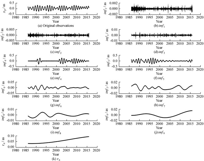
3.2 Separation of the low-and high-frequency oscillations in pole coordinatesTaking the xp pole coordinate as an example, Fig. 2 shows the decomposed results of the 30-year xp pole variations from January 1, 1986 to December 31, 2015. It can be seen in Fig. 2 that the xp pole coordinate can be decomposed into a limited number of IMFs using the EMD algorithm, indicating that the oscillations of different time-scale in the component of polar motion are characterized by a small number of IMFs. As can be found in Fig. 2, two of the modes, namely imf4 and imf5, show a noticeable seasonal oscillation in the range of a few hundreds of milliarcseconds, and thus can be considered as the two dominating oscillations along the x and y directions, namely annual wobble and Chandler wobble. In addition, we have found that the IMFs imf6, imf7, imf8 and imf9 with longer periods and the residuals rn arising from the EMD analysis can be identified as the inter-annual and inter-decadal signals and the long-term "natural" trend in the observations, and the modes imf1, imf2 and imf3 with the smaller amplitudes represent the shorter-period oscillations and the very high-frequency non-wobbling components. It is noteworthy that due to the mode mixing problem in the EMD the mode separation may be difficult when the signal contains components having adjacent periods, as it occurs for the Chandler and annual wobbles. Since here we only focus on separation of the low-and high-frequency oscillations rather than extraction of a particular component, however, this mode mixing problem dose not limit our analysis.
|
| Figure 2 Original xp pole coordinate and its IMFs arising from the EMD algorithm |
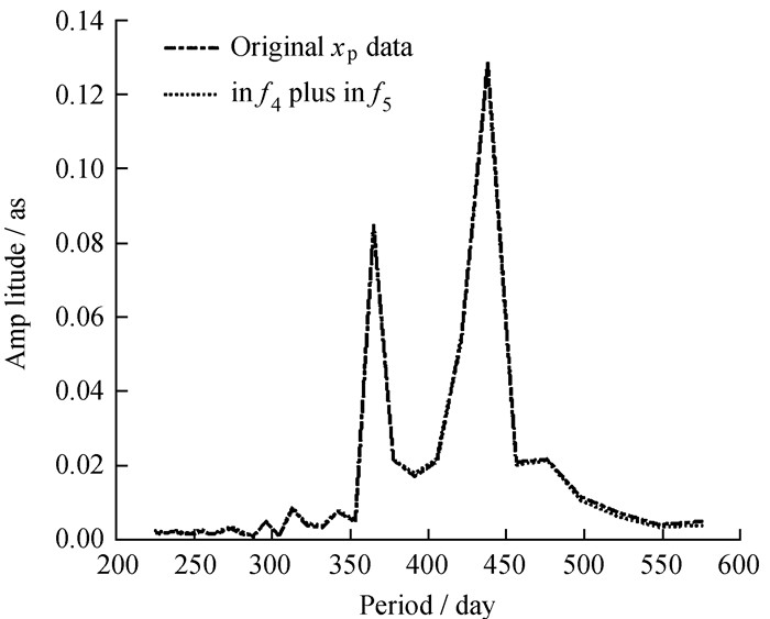
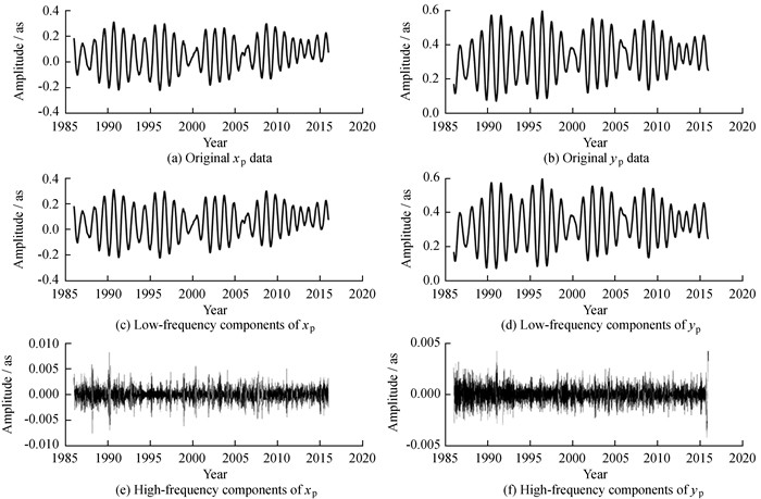
A spectral analysis of the IMFs imf4 plus imf5 based on fast Fourier transform (FFT) is exhibited in Fig. 3. In comparison, we also perform a similar analysis of the original data as given in Fig. 3. Visually, imf4 plus imf5 indeed contains the two dominant oscillating modes, i.e., Chandler and annual wobbles, with the same periods and amplitudes as the original observations do. Therefore, these finds confirm that the oscillating feature hidden in polar motion can be visually characterized by some oscillatory IMFs having particular physical meaning. To extract the high-frequency components of pole coordinates the IMFs imf1, imf2 and imf3 are reconstructed, while the other modes are counted up to gain the low-frequency oscillations including the long-term trend, Chandler and annual wobbles. Fig. 4 depicts the separated low-frequency time-series, high-frequency time-series of the xp, yp pole coordinates as well as the raw data. Their plots in Fig. 4 suggest that the low-frequency components including the Chandler wobble, annual wobble and long-term trend can be described by a low-order polynomial and harmonic model, while the AR technique is suitable for modelling the high-frequency terms.
|
| Figure 3 Spectral analysis of the oscillatory IMFs and original xp pole coordinates |
|
| Figure 4 Original xp, yp pole coordinates, the low-and high-frequency components |
EOP 08 C04 series serve as data basis and the length of base data is 10 years. The predictions of xp, yp pole coordinates are generated by means of the two prediction schemes: LS+AR and EMD+LS+AR. The length of all predictions is equal to 365 days.In order to compare with the official predictions from the IERS Bulletin A, which contains EOP predictions for 1 year into the future at daily intervals and is issued by the IERS Rapid Service/Prediction Centre at the U. S. Naval Observatory (USNO), all 365-day predictions of pole coordinate data are calculated every week at different starting prediction epochs from January 7, 2011 to December 31, 2015 because the IERS Bulletin A gives an advanced solution updated weekly.The comparison of the polar motion predictions is carried out by means of the analysis of: (1) the absolute values of differences between the pole coordinate data from the EOP 08 C04 series and their forecasts, and (2) mean absolute error (MAE) prediction errors defined by the following[6]
| $ MAE\text{ }\left( q \right)=\frac{1}{l}\sum\limits_{j=1}^{l}{\left| {{O}_{{{t}_{j}}+q}}-{{F}_{{{t}_{j}}+q}} \right|} $ | (10) |
where tj is the starting prediction epoch, l is the number of q-step predictions, Ftj+q is the q-step prediction of polar motion and Otj+q is the corresponding observation of the IERS EOP C04 series. In our analysis, q=1, …, 365.
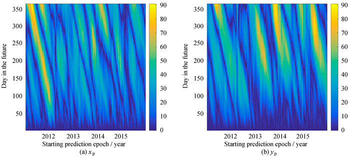
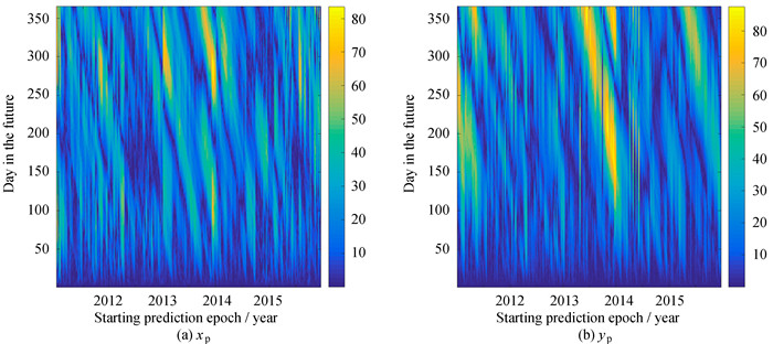
The maximum absolute values of the differences between the pole coordinate data and their LS+AR predictions calculated at different starting epochs exceed 98 mas.The larger differences are for the selected polar motion forecasts with predictions lengths greater than 5 months (Fig. 5). In the case of the polar motion predictions published by the IERS Bulletin A, the maximum values of the differences between the data and IERS predictions do not exceed 91 mas and those differences are smaller than those computed for our LS+AR scheme (Fig. 6). For the tested data span, the combination of the EMD and LS+AR model produces polar motion predictions with maximum absolute differences of less than 87 mas and the extreme perturbations are significantly smaller than for the LS+AR and IERS solutions (Fig. 7).

|
| Figure 5 Absolute differences (in mas) between the pole coordinate data and their LS+AR predictions calculated at different starting epochs |
|
| Figure 6 Absolute differences (in mas) between the pole coordinate data and their IERS predictions calculated at different starting epochs |
|
| Figure 7 Absolute differences (in mas) between the pole coordinate data and their EMD+LS+AR predictions calculated at different starting epochs |
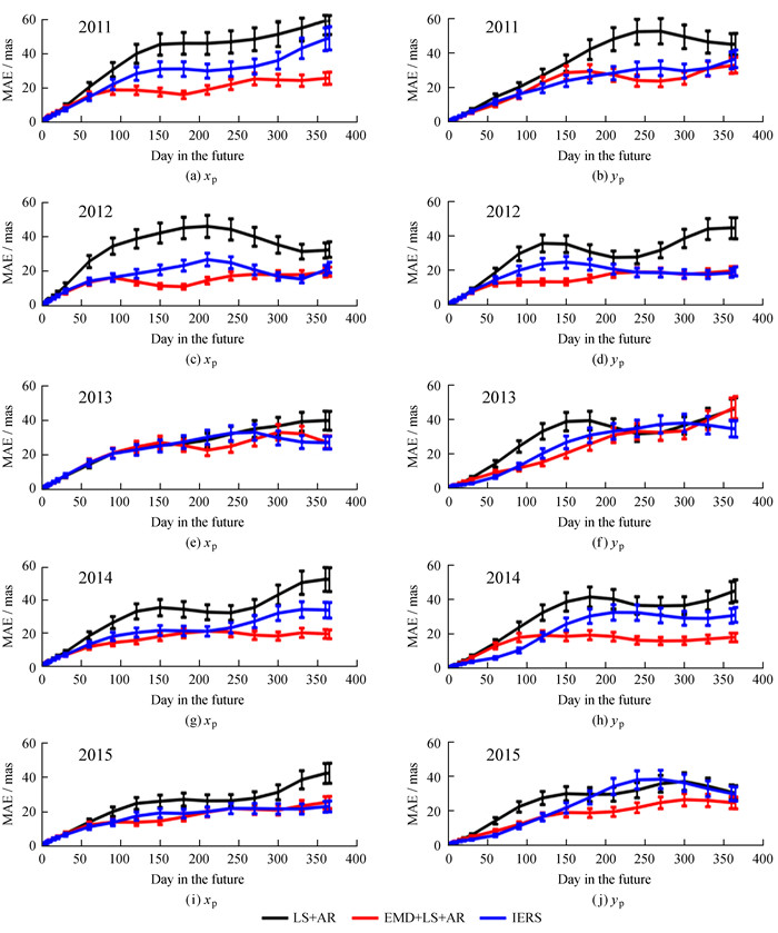
The representative statistic MAE as well as the corresponding error bars for our predictions in comparison with those for the IERS official predictions are shown year-by-year in Fig. 8. The results indicate that the accuracy of the LS+AR combination can be remarkably improved by incorporating the EMD into the prediction model, especially in long-term predictions. In contrast to the IERS predictions, our results obtained by the EMD+LS+AR approach appear to be comparable with those from the IERS for near-term prediction. However, for long-term prediction the proposed method noticeably outperforms the IERS solutions except individual prediction days, as can be seen apparently in Fig. 8.
|
| Figure 8 MAE for the LS+AR, EMD+LS+AR and IERS predictions of pole coordinates from 1 to 365 days in the future as well as the corresponding error bars |
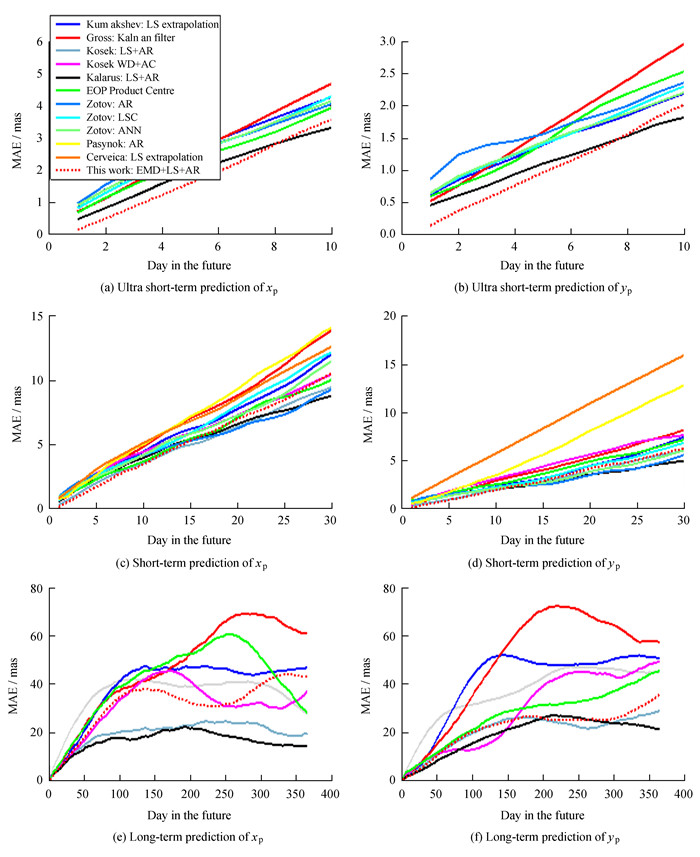
In order to furthermore demonstrate the effectiveness of the developed EMD+LS+AR prediction strategy, the results of this strategy are also compared with those from the EOP PCC lasting from October 1, 2005 to February 28, 2008, in which the prediction period and validation scheme had been clearly specified in advance. Under the same rules and conditions, the comparison with the contemporary prediction methods and techniques involved in the EOP PCC is shown in Fig. 9, in which the data time span is same, the statistics are referred to the EOP 05 C04 series and the MAE is used as the statistical measure. A list of participants and prediction methods can be found in [6].
|
| Figure 9 MAE for the EMD+LS+AR predictions and those contributed to the EOP PCC for different prediction days |
From the comparison it can be said that the error of the predictions for 1-10 days in the future by the EMD+LS+AR model is equal to the error of the most accurate prediction method for forecasting polar motion, namely the LS extrapolation of the harmonic model and AR prediction (Fig. 9(a)) and (Fig. 9(b)). For short-term (up to 30 days in the future) prediction, the prediction accuracy of the developed method is comparable with or slightly worse than the accuracy of the three most accurate prediction techniques used (Fig. 9(c)) and (Fig. 9(d)). As to long-term forecast, (up to 1 year in the future) the predictions are inferior to the most accurate results, in particular those of xp data. However, our results are significantly more accurate than the predictions contributed by the other participants (Fig. 9(e)) and (Fig. 9(f)).
4 Summary and conclusionOur investigations show that pole coordinate time-series were decomposed into a small number of IMFs representing different time-scale fluctuations, e.g., seasonal, inter-annual and inter-decadal fluctuations. Therefore, the EMD can be considered as a filter to extract specific oscillatory signals in polar motion. For the purpose of separation treatment of different components in time-series prediction, the EMD is used as a filtering method for separating the low-and high-frequency components of pole variations in our work. The results have indicated that both the shorter-period high-frequency variations and the low-frequency oscillations including the long-term trend, Chandler and annual wobbles can be extracted through reconstruction of the partial IMFs. Based on the findings, the LS extrapolation of the low-order polynomial and harmonic model and AR technology are recommended to predict the determined low-frequency and high-frequency components, respectively. The predictions of polar motion are generated by means of the combination of LS extrapolation and AR prediction. In order to evaluate the prediction accuracy of the proposed strategy, we have calculated the developed EMD+LS+AR as well as LS+AR predictions year-by-year at different starting prediction epochs between January 7, 2011 and December 31, 2015 in comparison with the IERS official forecasts. The figures of the MAE and absolute values of differences between pole coordinate data and their predictions illustrate that the presented hybrid approach indeed provides the more accurate predictions more than the conventional LS+AR combination, implying that the performance of the LS+AR method can be enhanced by involving the EMD into prediction model.Our results gained by the proposed method are better than the predictions released by the IERS as well, although those for individual prediction days are exception. In addition, the comparison between our results and the forecasts from the EOP PCC confirms that the EMD+LS+AR combination is a very powerful tool to predict pole coordinate data. The main conclusion is that the prediction error can be decreased when the EMD is incorporated into the LS+AR combination. Furthermore, we conclude that the separation treatment of different time-scale oscillations may enhance polar motion predictions and thus such processing seems to be of necessity in time-series prediction.
| [1] | Gambis D, Luzum B. Earth rotation monitoring, UT1 determination and prediction[J]. Metrologia, 2011, 48(4): 65–170. |
| [2] | Xu X Q, Zhou Y H. EOP prediction using least square fitting and autoregressive filter over optimized data intervals[J]. Advances in Space Research, 2015, 56(10): 2248–2253. DOI: 10.1016/j.asr.2015.08.007 |
| [3] |
雷雨, 蔡宏兵. 顾及最小二乘拟合端点效应的日长变化预报[J]. 天文研究与技术, 2016, 13(4): 441–445 Lei Yu, Cai Hongbing. Enhancing the prediction accuracy of the length of day change by eliminating the edge-effect of least squares fitting[J]. Astronomy Research & Technology, 2016, 13(4): 441–445. |
| [4] | Liao D C, Wang Q J, Zhou Y H, et al. Long-term prediction of the Earth orientation parameters by the artificial neural network technique[J]. Journal of Geodynamics, 2012, 62: 87–92. DOI: 10.1016/j.jog.2011.12.004 |
| [5] | Lei Yu, Cai Hongbing, Zhao Danning. Effects of training patterns on predictions of variations of length of day using an extreme learning machine neural network[J]. Astronomy Research and Technology, 2015, 12(3): 299–305. |
| [6] | Kalarus M, Schuh H, Kosek W, et al. Achievements of the Earth orientation parameters prediction comparison campaign[J]. Journal of Geodynamics, 2010, 84(10): 587–596. |
| [7] | Kosek W. Future improvements in EOP prediction[J]. Geodesy for Plant Earth, International Association of Geodesy Symposia, 2011, 136: 513–520. |
| [8] | Huang N E, Wu Z H. A review on Hibert-Huang transform:method and its application to geophysical studies[J]. Reviews of Geophysics, 2018, 46(2): 1–23. |
| [9] | Akaike H. Autoregressive model fitting for control[J]. Annals of the Institute of Statistical Mathematics, 1971, 23: 163–180. DOI: 10.1007/BF02479221 |
| [10] | Bizouard C, Gambis D. The combined solution C04 for Earth orientation parameters consistent with international terrestrial reference frame 2005[J]. International Association of Geodesy Symposia, 2009, 134: 265–270. DOI: 10.1007/978-3-642-00860-3 |
2. 中国科学院大学, 北京 100049;
3. 中国科学院时间频率基准重点实验室, 陕西 西安 710600


