 2016, Vol. 59


2 Institute of Statistical Mathematics, 10-3 Midori-Cho, Tachikawa, Tokyo 190-8562, Japan
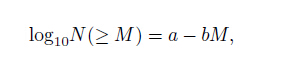
Earthquake catalogs are important datasets to understand seismicity, earthquake physics and earthquake hazard (Huang et al., 1994; Liu et al., 1996; Xu and Gao, 2014). For example, the b value calculated from a catalog can be a stress metric that inversely describes the differential stress (Schorlemmer et al., 2005). Other examples are aftershock sequences analyses (e.g. Woessner et al., 2004; Tan et al., 2015) and dynamic triggering phenomena analyses (e.g. Stein, 1999; Jia et al., 2012, 2014). Previous studies (Ishimoto and Iida, 1939, Gutenberg and Richter, 1944) show that the magnitude and the occurrence frequency of earthquakes follow:
|
(1) |
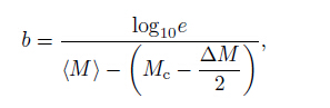
where N(≥ M) is the occurrence frequency of events of magnitude larger than or equal to M ; a and b, respec- tively, describe the background earthquake rate and the relative difference between small and large earthquakes. From the viewpoint of hazard assessment perspective, an accurate and robust estimation of the b value is es-sential. Aki (1965) introduced the following estimate:
|
(2) |
where (M) is the mean magnitude of the catalog with magnitude equal to or larger than Mc, ∆M is the width of the magnitude bin which is often set to be 0.1. From the equation above, a correct estimate of b is dependent on Mc.
Since earthquake signals are recorded by a monitoring network that might be spatially and temporally heterogeneous and possibly processed in various ways, it is essential to assess the quality and consistency of an earthquake catalog before using it for seismicity analysis. The changes in network distribution and number of sensors over time will change Mc of a catalogue. As for the deviations from Gutenberg and Righter (G-R) law at the lower end of the magnitude, incompleteness is caused by the following four factors:(1) The event is too small and its signal is undistinguishable from the background noise;(2) The magnitude is too small to be recorded by enough stations;(3) The network operator decides that events with magnitude under a certain threshold are not to be processed;(4) Small events are hard to be detected from the coda of a possible aftershock sequence (Mignan and Woessner, 2012). The above four factors contribute to a detection rate that gradually increases with the magnitude and ends up at 100% above a certain magnitude. A cumulative probability function is commonly used to describe the gradually changed detection capability (e.g. Ogata and Katsura, 1993, Iwata, 2008).
Mc is usually defined as the lowest magnitude at which the earthquakes in a space-time volume are 100% detected (Rydelek and Sacks, 1989). In practice, Mc acts as the cutoff magnitude for choosing a subset from a real recorded catalog for seismic analysis. In this study, we focus on finding the optimal method to give a valid Mc estimation for selecting a subset catalog. Assuming that earthquake process is self-similar, the earthquake frequency-magnitude distribution (FMD) should be consistent with the G-R Law (Eq.(1)). The deviations from theoretical linear prediction at large magnitude may due to random fluctuations because of the scarcity of large events or the characteristic earthquake phenomenon (Schwartz and Coppersmith, 1984) and at the low end the deviations are explained by the deficiency of detection capability of networks as mention before.
Shown in Eq.(2), the estimated b value for a given catalog is dependent on the cutoff magnitude Mc. To calculate b value correctly, a subset must be selected to assure that events are 100% or close to 100% detected. An erroneously lower Mc value may lead to erroneous seismicity parameter values and bias the analysis because of the incompleteness of a catalog. A ‘safe’ way to assure the completeness is to choose a larger than optimal Mc value. However, this leads to less usable data. The trade-off between assuring 100% detection and usable data is an important thing to consider in this study.
This study evaluates the performances of different catalog-based methods in estimating Mc by numerical tests on synthetic catalogs, we hope to provide guidelines for selecting the optimal Mc estimation method case to case. There are two main types of methods for estimating Mc: the first one is catalog-based, which only uses catalog data. The second one is waveform-based that uses waveform data to calculate signal-to-noise ratio (e.g.Sereno and Bratt, 1989, Gomberg, 1991) or phase-pick data. Most of these techniques estimate a general Mc in a space-time volume. However, Probability-based Magnitude of Completeness (PMC) developed by Schorlemmer and Woessner (2008) and Bayesian Magnitude of Completeness (BMC) developed by Mignan et al.(2011) can estimate Mc varying with time and space. For example, Li and Huang (2014) adopted the PMC method to estimate detectability of the Capital-circle Seismic Network. The catalog-based techniques are less expensive and less time-consuming than the waveform-based techniques (Woessner, 2005). There are many studies using this type of methods to estimate Mc in China (e.g. Li et al., 2011; Feng et al., 2012). We consider five popular catalog-based methods in this study:
(1) The Maximum Curvature (MAXC) technique (Wiemer and Wyss, 2000)
The Maximum Curvature technique computes the maximum value of the first derivative of the frequency- magnitude curve. This matches the magnitude with the highest frequency of events in the non-cumulative frequency magnitude distribution (FMD) in practice. This method is time-saving and easy-handling.
(2) The Goodness-of-Fit Test (GFT)(Wiemer and Wyss, 2000)
The Goodness-of-fit test (Wiemer and Wyss, 2000) evaluates the differences between the observed FMD and the synthetic ones. Large difference means low goodness of fit, when the incomplete part is included. In the procedure, first, for each magnitude threshold Mc0, theoretical distribution from the G-R law is calculated with the maximum likelihood estimation of the a and b value from observations. Then the absolute difference R of events in each magnitude bin between the observed and theoretical distribution can be calculated:

|
(3) |
where Bi and Si are the observed and predicted cumulative numbers of events in each magnitude bin. Mc is decided as the smallest magnitude cutoff Mc0 where R achieves the confidence level e.g. 90% or 95%. When 95% confidence level can be satisfied, a 90% level is a compromise.
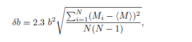
(3) The Mc by b value stability (MBS) approach (Cao and Gao, 2002) The Mc by b value stability is proposed by Cao and Gao (2002), which regards the stability of b value as a function of magnitude threshold Mc0. The basic assumption of this method is that b value increases as Mc0 approaching Mc, and remains constant for Mc0 ≥ Mc. The criterion for b value stability in Cao and Gao (2002) is defined as 0.03, a value which is not always stable. Woessner and Wiemmer (2005) improve the method by using a b value uncertainty δb (Shi and Bolt, 1982):
|
(4) |
where (M) is the mean magnitude of events whose magnitude is larger than Mc0 , and N is the number of events. Mc is then defined as the smallest magnitude satisfying ∆b = |bave - b| ≤ δb. The ∆m is calculated from the b-values of successive magnitudes from Mc0 to Mc0 + dM, where ∆m is the bin size 0.1 and dM is 0.5.
(4) The Median-based Analysis of the segment slope (MBASS)(Amorese, 2007)
The Median-Based Analysis of Segment Slope of Amorese (2007) is based on an iterative method to search for multiple changes in a non-cumulative FMD. It first calculates a segment slope series between two consecutive magnitude points. With the initial series, the segment slope subtracts the median of the series at each iteration. At each iteration, a Wilcoxon-Mann-Whitney (WMW) test (Mann and Whitney, 1947, Wilcoxon, 1945) was applied to find a significant and stable change in the median of segment slope which corresponds to Mc.
(5) Mc from the Entire Magnitude Range (EMR) (Woessner and Wiemer, 2005)
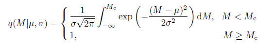
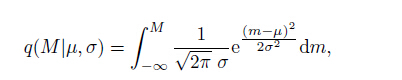
The Entire Magnitude Range method proposed by Woessner and Wiemer (2005) sets a model consisting of two parts: the G-R law for the complete part and a cumulative normal distribution function q(M |µ, σ) describing the detection capability to fit the incomplete part. The detection capability function q(M |µ, σ) at magnitude M can be expressed as
|
(5) |
where µ is the magnitude at which 50% of the earthquakes are detected and represent the detectability of a seismic network. σ is the standard deviation representing the magnitude range width of partial detection which describes how fast the detection capability changes with earthquake magnitude. The larger σ, the more slowly detection capability changes with magnitudes. Because Mc is explicit in Eq.(5), it can be estimated with the maximum likelihood function of observed earthquake probability density.
This study aims to test how these catalog-based methods behave on estimating Mc under different condi-tions. In the following, we use 3 models to see how the change rate of detection capability with magnitude in the incomplete part, the event number and the heterogeneity influence the estimation of Mc. With numerical tests on the five methods, advantages and pitfalls of them are discussed.
2 GENERATIONS OF THE SYNTHETIC CATALOGUESThe synthetic catalogs are generated following Ogata and Katsura’s (1993) model (marked as OK1993 here-after). The detection rate function for describing earthquake detectability is the cumulative normal distribution following Eq.(6):
|
(6) |
where the parameters have the same meanings as in Eq.(5). Both Woessner & Wiemer (2005) and OK1993 use the cumulative normal distribution function to describe the detection rate, but the former was only applied to the incomplete part and the latter was implemented to the whole magnitude range. As shown by Woessner & Wiemer (2005), among the cumulative distribution functions used to fit lots of real catalogs, the cumulative normal distribution function fits the data best. We decided to use OK1993 instead of Woeesner & Wiemmer’s model to generate synthetic catalogs for that the earthquake detection ability changes gradually with magnitude and discontinuity is unreasonable in the detection progress. Rejection method (see e.g. Zhuang and Touati, 2015) is adapted to the stochastic simulation of earthquake catalogs. In the simulation process, we first derive the observed probability density function λ(M) by multiplying the theoretical distribution of magnitude λ0(M) and detection rate q (M) and then normalize q (M)λ0(M). Based on the G-R law shown in Eq.(1), the theoretical distribution of magnitude is
|
(7) |
where β = b ln10. The observed normalized probability density can be written as follows
|
(8) |
Three models are used in our simulations. In the first model (marked as Model 1 hereafter), the earthquake probability density follows Eq.(8), with b = 0.9, µ = 1.5 and σ = 0.2 in q(M). We set b to be 0.9 for b is often 0.8∼1.1 in real catalogs. σ is set to be 0.2 in accordance with former studies. µ describes the detectability of a network. µ equaling 1.5 shows that there is 50% possibility to record and locate an M = 1.5 earthquake.Because Mc is relative to µ, the choice of µ does not influence the results of this study. The parameters in the second model (marked as Model 2 hereafter) is the same as Model 1 except σ = 0.4, which means the detection capability of networks changes slower with magnitude. In Model 3, a catalog generated from Model 1 is combined with an equal event number catalog with magnitude above 1.5 100% recorded. The catalogs generated from Model 1 or Model 2 belong to homogeneous catalogs. In Model 1 and Model 2, σ describes how fast the detection rate changes with magnitude. When σ goes to infinity, it means the network has equal detection rate for all the earthquakes with different magnitudes. Considering that Model 1 and Model 2 cannot represent the case of today’s real catalogs as detection capability improves with time, we use Model 3 to test the effects of temporal heterogeneities. The probability densities for Models 1, 2 and 3 are respectively illustrated from Figs. 1a to Figs. 1c.
Five magnitudes at which one event is expected to be unrecorded in every 100, 500, 1000, 5000 and 10000 events in 3 models are listed in Table 1 as possible criterions for Mc. These magnitudes can be calculated by solving the following equation:
|
(9) |
|
|
Table 1 Possible theoretical criterion for Mc |
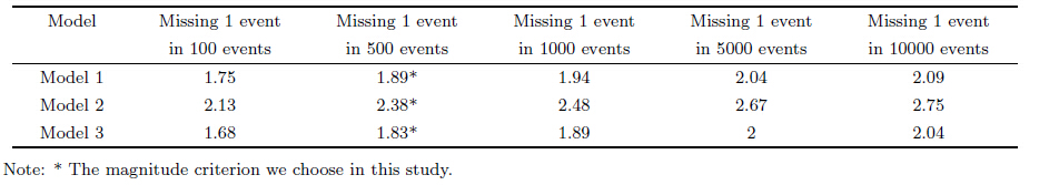
where N is the total event number, q (m)is the detection rate shown in Eq.(6). These Mc criterions are shown in Table 1 as well as illustrated in Figs. 1a to Figs. 1c. We choose the magnitude at which one event is expected to be unrecorded in every 500 events as the criterion for Mc in this study. Because the magnitude recorded in most real catalogs only preserves one decimal, the Mc criterion is correspondingly rounded to one decimal 1.9, 2.4 and 1.8 respectively for Models 1 to 3. To study the effects of choosing Mc on b value and goodness of fit, we use 100 catalogs, each with 2cjg-59-3-266 events generated from 3 models, to calculate mean b values and mean goodness of fit defined by Eq.(3) from Mc 1.5 to 3. The b values and goodness of fit defined by Eq.(3) together with the Mc criterions we choose are illustrated in Fig. 2. Results of all tests will be compared with the Mc criterion we choose. Readers can choose other criterions for Mc according to their tolerance of missing earthquake events and compare the test results.

|
Fig. 1 Probability density function of three models for simulation |

|
Fig. 2 Mean b value and goodness of fit corresponding to different Mc |
For each of the above three models, we simulated 3 groups of catalogs, each group including 1000 synthetic catalogs. The difference among the 3 groups is the number of events in each catalog: there are 10000 events in each synthetic catalog for Group 1, 50000 events for Group 2, and 1cjg-59-3-266 events for Group 3. In the coming section, we apply the Mc estimation methods to these synthetic catalogs and compare their behaviors.
3 TESTS ON Mc DETECTIONFive methods introduced above are used to estimate the Mc of 9 groups of synthetic catalogs generated from three models. The results are discussed in this section as follows.
(1) MAXC. From Figs. 3a to 3c, the estimated Mc for Groups 1 to 3 are almost equally distributed on 1.6 and 1.7 which is underestimated compared to 1.9. This method is not event-number dependent for the distributions of Mc slightly change when event number increases. When standard deviation σ increases to 0.4, the variance of the estimated Mc increases correspondingly and the estimated Mc decreases mainly to 1.5 or 1.4(Figs. 3d to Figs. 3f) which is far below 2.4. Because the events are more widely discarded and the magnitude of most events is more likely to diverge from Mc, this method behaves worse when the detection capability changes slowly with magnitude. When implemented to mixed catalogs, the estimated Mc is always 1.6, lower than 1.8(Figs. 3g to Figs. 3i). We conclude that when implemented to a homogeneous catalog, MAXC tends to underestimate Mc for the results in Model 1 and Model 2 are significantly lower than the Mc criterion we choose in Table 1. However, this method can achieve a stable estimation with a small volume of events. MAXC is not valid when implemented to heterogeneous catalogs generated by Model 3.

|
Fig. 3 Estimation results of 5 methods |
Our result differs a bit from Mignan et al.(2011) which suggests the underestimation is due to spa- tiotemporal heterogeneities of a network. In our homogenous models, the estimation of Mc is also significantly underestimated. This underestimation may be caused by the algorithm which chooses the magnitude with the most events. With the magnitude increasing, the possibility of events detection is increasing but the G-R law indicates that the occurrence of events is decreasing. The trade-off between them could explain why Mc may not correspond to the magnitude with the most events. The fact that the underestimation of Mc is relevant to the change rate of a network’s detection capability with magnitude also supports our viewpoint.
(2) GFT. As the goodness of fit for the synthetic catalogs can achieve 95% confidence level, we choose the 95% confidence level as the criterion of Mc estimation. The Mc distribution and cumulative probability are shown by the lines marked with triangle in Fig. 3. From Figs. 3a to Figs. 3e, we can see that the Mc estimation values converge to 1.6 and 1.7 for Models 1 and 2 respectively with the increasing event number. The results shown in Figs. 3g to Figs. 3i for Model 3 have a major value 1.6 and a minor value 1.5. When the event number is increased, the results become more stable. This method behaves better than MAXC when the network’s detection capability changes slowly with magnitude and catalogs have heterogeneity. But for all three models, this method underestimates Mc as MAXC does.
A possible explanation for underestimation is that this method chooses the lowest magnitude cutoff at which the confidence level is achieved and omits all the magnitudes that achieve the confidence level. A higher confidence level is preferred when it can be achieved for it provides estimation closer to the true value. Compared with MAXC, GFT is more resistant to heterogeneity and the change rate of a network’s detection capability with magnitude for GFT uses all the events above a certain magnitude threshold.
(3) MBS. We tested improved MBS (Woessner and Wiemer, 2005) using ∆b = |bave - b| ≤ δb as the criterion. The standard deviation δb is calculated by 100 times’ bootstrap which is time-consuming. Compared to other methods, MBS almost has the highest Mc estimation. A characteristic of this method is that the estimation of Mc has a long range tail. In Figs. 3a to Figs. 3c, the estimated Mc’s main value changes from 1.8 to 1.9 with increasing event number which is just the Mc criterion. Figs. 3d to Figs. 3f show the Mc estimated by this method is the most sensitive to the change rate of a network’s detection capability with magnitude. With the increasing event number, the estimated main value for Model 2 changes from 2 to 2.1 and has a certain probability to be 2.2 or 2.3, slightly lower than 2.4. When applied to the synthetic catalogs from Model 3, the estimated values of Mc are mainly 1.8 which is the Mc criterion for Model 3, and sometimes 1.9(Figs. 3g to Figs. 3i).
We conclude that this method is time-consuming but relatively conservative. The estimated results for Models 1 and 3 are just the criterion for Mc. For Model 2, the estimated Mc is the highest though lower than the criterion 2.4. But this method needs a relatively large event number to achieve a stable estimation.
(4) MBASS. MBASS is also an event number dependent method and also needs a large number of events to obtain stable estimation of Mc. Figs. 3a to Figs. 3c show that the main estimated values increased from 1.8 to 1.9 with the increasing event number. When the network’s detection capability changes more slowly with magnitude, it can be obviously seen from Figs. 3d to Figs. 3f that the results become more dependent on the event number. The main value of Mc estimation for Model 2 changes from 1.6 gradually to 1.9 when the event number increases. As to the mixed catalogs, MBASS gives similar results as MBS with a main value 1.8(Figs. 3g to Figs. 3i).
This method works well when the detection capability changes rapidly with magnitude or heterogeneity exists. The estimated Mc is just the Mc criterion when the number of events is large. This method is much less time-consuming compared with MBS. When the detection capability of a network changes slowly with magnitude, this method gives larger Mc estimation than all methods except MBS, but the Mc value is still underestimated.
(5) EMR. The main estimated Mc value for Model 1 is consistently 1.7 as shown in Figs. 3a to Figs. 3c. When the detection capability changes slowly with magnitude, the variance of the estimated Mc becomes larger as shown in Figs. 3d to Figs. 3f. The results for Model 2 indicate that this method is not sensitive to the change rate of a network’s detection capability with magnitude since the main estimated value is still 1.7(Figs. 3d to Figs. 3f). When implemented to synthetic catalogs in Model 3, this method estimates the Mc to be 1.5 or 1.6 with almost the same probability (Figs. 3g to Figs. 3i). This method does not need many events to achieve a stable estimation but it tends to underestimate Mc in all models. Compared with other 4 methods, EMR often gives moderate Mc estimation which is larger than MAXC&GFT but smaller than MBASS&MBS. Catalogs with incomplete part does not assume cumulative normal distribution are not tested but we speculate it may be less effective.
4 DISCUSSIONSMc is underestimated by all 5 methods when the standard deviation σ becomes 0.4, so we suggest that when detection capability changes gradually with magnitude the catalogs should be coped with care. For catalogs with heterogeneity and recorded by a network whose detection capability changes slowly with magnitude, we recommend MBASS when the event number is large enough for the Mc estimation. When the detection rate of a network improves slowly with magnitude, MBS is recommended if time is not limited and large number of events are available.
The synthetic catalog models of this study are based on OK1993. The OK1993 model has its advantages as mentioned before, but the test is less definite with the EMR method for using the same probability function in the incomplete part. Other models need to be considered to simulate the incomplete part of the catalogs for testing EMR, but we suspect this method will be less effective. Because the choice of normal cumulative distribution function is not based on physical process, possibility exists that other functions might be more suitable.
Our conclusion on EMR differs from Woessner and Wiemer (2005). They compared EMR with MAXC, GFT and MBS, and found that EMR showed a superior performance in estimating Mc, but in this study we think this method underestimates Mc and gives a moderate estimation of Mc between MAXC&GFT and MBASS&MBS. In their synthetic catalogs, events with magnitude larger than 1.5 is completely detected. This leads to discontinuity as mentioned before. We have applied EMR to catalogs whose detection probability above a certain magnitude is 1, and find EMR actually behaves well. Another concern is that Woessner and Wiemer (2005) consider the relationship between the uncertainty of Mc and event number, finding the EMR method needs the least number to achieve a small variance of estimated Mc. We agree that EMR is superior considering this aspect. We think the reason leading to EMR underestimating Mc is that this method adopts a Kolmogorov-Smirnov test at 0.05 significance level to examine the goodness-of-fit between the EMR model and the actual data. The null hypothesis H0 is that the two samples are drawn from the same distribution. This method can be viewed as a two-part GFT method which uses two functions to fit the complete and incomplete part respectively. Thus, we think this method has the same pitfalls as GFT to underestimate Mc for choosing the first magnitude threshold as Mc when the significance level is satisfied. The underestimation of estimated Mc is relevant to the significance level. Another possible reason for underestimation is that if the goodness of fit of the complete part is high, the goodness of fit of the incomplete part will be relatively low which will bias the estimation of Mc.
Some Mc estimation methods do not rely on a large number of events, but some do. In our numerical tests, we generated whatever large number of events we need. It is not always the case in the real recorded catalogs. When limited events are available, bootstrap is used to increase the stability of Mc estimation. The difference between bootstrap and generating events from a model needs to be investigated. If the difference is small, the conclusion of this study can be applied to practice. We can increase event number in the real catalog and apply the more event-number reliable method to them.
5 CONCLUSIONSNot only the Mc represents the detection ability of a network, but it is also used to select a subset catalog for b value and a value estimation. The influence of a selected subset catalog can be seen from Figs. 2a and 2b. We can see that the criterion we choose is reasonable considering b value and goodness of fit.
We have compared the results from each method with the Mc criterions we choose from Table 1 and conclude the advantages and pitfalls of each methods as follows.
(1) MAXC is easy and inexpensive to perform but underestimates the Mc. This method can achieve a stable estimation with few events. This method does not work well with heterogeneous catalogs, so it is not recommended to cope catalogs with heterogeneity. When the detection capability changes more slowly with magnitude, underestimation increases by 0.2 or 0.3 in this study. We suggest to add an Mc correction according to the change rate of detection capability when implementing this method.
(2) GFT underestimates Mc as MAXC does, but more stable and resistant to heterogeneity than MAXC. This method is time-saving and event number independent. An Mc criterion should be added according to the change rate of detection capability when using this method.
(3) MBS behaves well for all three models though underestimates Mc slightly when detection capability changes slowly with magnitude. This method needs more events to become stable and is time-consuming compared to other methods. This method is recommended when the amount of events is large enough and time is not limited.
(4) MBASS can estimate Mc correctly for catalogs with enough events when the detection capability changes rapidly with magnitude and heterogeneity exits. When the detection capability changes slowly with magnitude, this method is not comparable to MBS. Therefore, this method is suggested instead of MBS when the network’s detection capability changes rapidly with magnitude and catalogs contain heterogeneity.
(5) EMR underestimates Mc in all cases and it is not sensitive to the change rate of a network’s detection capability with magnitude. As EMR is based on a four-parameter estimation, this method is relatively stable and not event number dependent but more time-consuming than other method except MBS in our tests. This method gives a moderate estimation of Mc between MAXC&GFT and MBASS&MBS. Therefore, when we need a stable estimation while the event number is not large, this method is recommended if we have a relatively high tolerance for missing earthquake events. A rational criterion can be added to Mc.
AcknowledgeWe thank two anonymous reviewers for their constructive advice. This work was supported by the Special Fund for Earthquake Science Research in the Public Interest (2014419013) and the National Natural Science Foundation of China (41474033). We thank Prof. Woessner for discussion with the programs of calculating Mc. We would like also thank Mr. Wenyuan Fan for his constructive suggestions.
| [1] | Aki K. 1965. Maximum likelihood estimate of b in the formula and its confidence limits[J]. Bull. Earthq. Res. Inst., 43 : 237–239. |
| [2] | Amorese D. 2007. Applying a change-point detection method on frequency-magnitude distributions[J]. Bull. Seismol. Soc. Am., 97 (5): 1742–1749. |
| [3] | Cao A M, Gao S S. 2002. Temporal variation of seismic b-values beneath northeastern Japan island arc[J]. Geophys. Res. Lett., 29 (9): 48–1. |
| [4] | Gomberg J. 1991. Seismicity and detection/location threshold in the southern Great Basin seismic network[J]. Journal of Geophysical Research:Solid Earth (1978-2012), 96 (B10): 16401–16414. |
| [5] | Gutenberg B, Richter C F. 1944. Frequency of earthquakes in California[J]. Bull. Seismol. Soc. Am., 34 (4): 185–188. |
| [6] | Ishimoto M, Iida K. 1939. Observations of earthquakes registered with the microseismograph constructed recently[J]. Bull. Earthq. Res. Inst., 17 : 443–478. |
| [7] | Iwata T. 2008. Low detection capability of global earthquakes after the occurrence of large earthquakes:Investigation of the Harvard CMT catalogue[J]. Geophys. J. Int., 174 (3): 849–856. |
| [8] | Jia K, Zhou S, Wang R. 2012. Stress interactions within the strong earthquake sequence from 2001 to 2010 in the Bayankala block of eastern Tibet[J]. Bull. Seismol. Soc. Am., 102 (5): 2157–2164. |
| [9] | Jia K, Zhou S Y, Zhuang J C, et al. 2014. Possibility of the independence between the 2013 Lushan earthquake and the 2008 Wenchuan earthquake on Longmen Shan fault, Sichuan, China[J]. Seismol. Res. Lett., 85 (1): 60–67. |
| [10] | Mann H B, Whitney D R. 1947. On a test of whether one of two random variables is stochastically larger than the other[J]. The Annals of Mathematical Statistics, 18 (1): 50–60. |
| [11] | Mignan A, Werner M J, Wiemer S, et al. 2011. Bayesian estimation of the spatially varying completeness magnitude of earthquake catalogs[J]. Bull. Seismol. Soc. Am., 101 (3): 1371–1385. |
| [12] | Mignan A, Woessner J. 2012. Estimating the magnitude of completeness for earthquake catalogs. Community Online Resource for Statistical Seismicity Analysis, doi:10.5078/corssa-00180805. |
| [13] | Ogata Y, Katsura K. 1993. Analysis of temporal and spatial heterogeneity of magnitude frequency distribution inferred from earthquake catalogues[J]. Geophys. J. Int., 113 (3): 727–738. |
| [14] | Rydelek P A, Sacks I S. 1989. Testing the completeness of earthquake catalogues and the hypothesis of self-similarity[J]. Nature, 337 (6204): 251–253. |
| [15] | Schorlemmer D, Wiemer S, Wyss M. 2005. Variations in earthquake-size distribution across different stress regimes[J]. Nature, 437 (7058): 539–542. |
| [16] | Schorlemmer D, Woessner J. 2008. Probability of detecting an earthquake[J]. Bull. Seismol. Soc. Am., 98 (5): 2103–2117. |
| [17] | Schwartz D P, Coppersmith K J. 1984. Fault behavior and characteristic earthquakes:Examples from the Wasatch and San Andreas fault zones[J]. Journal of Geophysical Research:Solid Earth (1978-2012), 89 (B7): 5681–5698. |
| [18] | Sereno T J Jr, Bratt S R. 1989. Seismic detection capability at NORESS and implications for the detection threshold of a hypothetical network in the Soviet Union[J]. Journal of Geophysical Research:Solid Earth (1978-2012), 94 (B8): 10397–10414. |
| [19] | Shi Y L, Bolt B A. 1982. The standard error of the magnitude-frequency b value[J]. Bull. Seismol. Soc. Am., 72 (5): 1677–1687. |
| [20] | Stein R S. 1999. The role of stress transfer in earthquake occurrence[J]. Nature, 402 (6762): 605–609. |
| [21] | Wiemer S, Wyss M. 2000. Minimum magnitude of completeness in earthquake catalogs:examples from Alaska, the western United States, and Japan[J]. Bull. Seismol. Soc. Am., 90 (4): 859–869. |
| [22] | Wilcoxon F. 1945. Individual comparisons by ranking methods[J]. Biometrics Bulletin, 1 (6): 80–83. |
| [23] | Woessner J, Hauksson E, Wiemer S, et al. 2004. The 1997 Kagoshima (Japan) earthquake doublet:A quantitative analysis of aftershock rate changes. Geophys. Res. Lett., 31, doi:10.1029/2003GL018858. |
| [24] | Woessner J, Wiemer S. 2005. Assessing the quality of earthquake catalogues:Estimating the magnitude of completeness and its uncertainty[J]. B SeismolSoc Am., 95 : 684–698. |
| [25] | Zhuang J C, Touati S. 2015. Stochastic simulation of earthquake catalogs. Community Online Resource for Statistical Seismicity Analysis, doi:10.5078/corssa-43806322. |