 2016, Vol. 59


In a region extending from a height of about 60 km to 2000 km, most of the molecules of the atmosphere are ionized by the effects of solar high-energy electromagnetic radiation, cosmic rays and fallout particle. This region is called the ionosphere, which is an important part of the near earth space environment. The ionosphere contains enough free electrons and has a lot of effects on radiowaves propagation, especially on HF radiowaves(Felgate and Golley, 1971). These effects carry information about ionosphere regions. So, HF signals are often used to ionospheric real-time sounding for fully studying the structures, changes and disturbances of the ionosphere.
HF ionospheric vertical sounding(Hunsucker, 1991)is the oldest but still very important conventional ionospheric sounding means. Signals are sent straight up at many frequencies and after receipt they are usually displayed in terms of the ionospheric virtual height versus frequency, i.e. vertical ionogram. The vertical electron density profile(ionospheric height versus plasma frequency or electron density)can be inverted based on the extracted vertical echo trace using ionogram automatic scaling method(Reinisch and Huang, 1983; Galkin et al., 1996; Gilbert and Smith, 1988; Liu et al., 2009; Scotto and Pezzopane, 2004), and it can provide detailed information on ionospheric electron structures and changings, which are important to study the structures of the ionosphere, wave propagation and space weather applications. Therefore, the inversion of the vertical ionogram has gathered very wide attention all the time.
At present, the vertical ionogram inversion methods can be summarized as two categories: ① Direct calculation methods. These methods calculate the true heights directly from the measured virtual heights at a given series of frequencies, such as the lamination method(Titheridge, 1959), the single polynomial method(Titheridge, 1961)and the overlapping polynomial method(Titheridge, 1967), etc. Some of these methods calculate the true heights in one step by the simultaneous equations about the true and virtual heights, such as the lamination method and the single polynomial method. Some of them calculate the true heights step by step, beginning from the lowest frequency, such as the overlapping polynomial method, and the lamination method can also use this means. Titheridge(1985)developed the POLAN program for vertical ionogram automatic inversion based on the direct calculation methods. ② Model methods(Dyson and Bennett, 1988; Ding et al., 2007; Jiang et al., 2014; Reinisch and Huang, 1983; Scotto, 2009; Zheng, 1992). These methods assume that the electron density profile can be characterized by some kind of model, then determine its parameters by selecting the best-fit trace from the candidate traces that are synthesized by this model. Model methods don’t require perfect ionograms and provide good inversion results. They are widely used and scholars developed a variety of model-based inversion methods using different measured data.
Reinisch and Huang(1983)proposed a model-based profile inversion method using the shifted Chebyshev polynomials and developed the NHPC program which is included in the ARTIST system. In this method, the F layer profile is described by the shifted Chebyshev polynomials the coefficients of which are optimized in a least squares sense to best reproduce the measured trace. Considering that F1 layer trace obviously exists in the echo trace, some improvements have been made for the model, that is, the F1 and F2 layer are separately described by different shifted Chebyshev polynomials. This method is more suitable for completely developed case of the F1 layer. For incompletely developed case of the F1 layer, there would be some difference around critical frequency between the synthesized and measured traces, and not considering the profile smoothness at the joint between the F1 and F2 layer is also a shortcoming of this method.
The incompletely development of the F1 layer, means that the F1 layer profile at the peak is a finite slope. At this moment, a smooth transition from the F1 to the F2 layer, not a cusp at the critical frequency of the F1 layer, is usually seen on the vertical ionogram. This case often appears on vertical ionograms. Wang(2010)has also proposed the inversion method based on the QPS model when the F1 layer is incompletely developed. This paper studies mainly the incompletely developed case of the F1 layer, considering the smoothness of ionosphere profile, based on the ionosphere profile inversion method proposed by Reinisch and Huang(1983)and Reinisch et al.(1988), builds up the ionospheric model and describes the inversion process in details. Moreover, the proposed method is applied to the simulated and measured data for testing its effectiveness.
2 IONOSPHERIC MODEL FOR INCOMPLETELY DEVELOPED CASE OF THE F1 LAYERIn the existing commonly used ionospheric model, whether the QPS model(Dyson and Bennett, 1988), the IRI(international reference ionosphere)model(Bilitza, 1990), or the shifted Chebyshev polynomials model proposed by Reinisch and Huang(1983)and Reinisch et al.(1988), the electron density profile at the peak height of each layer is approximately in the parabolic shape, and the gradient of the profile here is infinite. It means that the lower layer achieves the maximum electron density and then enters the higher layer at the parabolic vertex, as shown in red solid line in Fig. 1a(red dotted line is shown as parabolic shape here). When the F1 layer is completely developed, the layer model mentioned above is appropriate. At this moment, the echo trace shows "moving upward" at the critical frequency of the F1 layer, and forming a cusp, as shown by the red solid line in Fig. 1b. However, for incompletely developed case of the F1 layer, the lower layer has reached the maximum electron density, and entered the higher layer, at the position not reaching the parabolic vertex, and the profile gradient is a finite number, as shown by the blue solid line in Fig. 1a(blue dotted line shows the parabolic shape here). At this moment, the echo trace is usually expressed as smooth transition from the F1 to the F2 layer, as shown by the blue solid line in Fig. 1b. For the incompletely developed case of the F1 layer, the commonly used models mentioned above would not sufficiently describe the changes of the profile.

|
Fig. 1 The diagram of the profile and the echo trace of incompletely developed F1 layer |
For the difference mentioned above between the profiles of completely developed F1 layer and the incompletely developed one, we introduce a parameter named as model setting critical frequency and establish an electron density profile model based on the shifted Chebyshev polynomials(Reinisch and Huang, 1983; Reinisch et al., 1988)for incompletely developed case of the F1 layer. The detailed description of the new model is as follows.
The new model contains the E, the valley, the F1, and the F2 four layers to describe the ionosphere profile. Parabolic profile shapes are assumed for the E layer and the valley. The F1 and F2 layers are approximated by the shifted Chebyshev polynomials. And the entire profile is given by:

|
(1) |
The connection point of the E layer and the valley is located at the peak height hmE of the E layer. The valley connects with the F1 layer at the height h2, where the plasma frequency equals to fCE, the critical frequency of the E layer. The valley consists of two joining segments: one connects with the E layer and the other connects with the F1 layer. The connection point of two joining segments is located at the height h1. The F1 layer connects with the F2 layer at the peak height hmF1 of the F1 layer. The meanings of symbols in(1)are as follows:
(1)The E layer:
fNE, fCE, hmE and ymE are the plasma frequency, the critical frequency, the peak height and the semithickness of the E layer, respectively. hbE = hmE - ymE denotes the base height of the E layer.
(2)The valley:
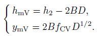
fNV, fCV and ymV are the plasma frequency, the minimum plasma frequency and the semi-thickness of the valley, respectively. hmV denotes the height where the plasma frequency of the valley equals fCV.h2 = hmE+W, where W is the valley width.
(3)The F1 layer:
Ti(g)are the shifted Chebyshev polynomials, which can be expressed as

|
(2) |
with

|
(3) |
fNF1 and fCF1 are the plasma frequency and the critical frequency of the F1 layer, Ai(i = 0 ~ I + 1)are the coefficients of the shifted Chebyshev polynomials, and

|
(4) |
hmF1 is the peak height of the F1 layer:

|
(5) |
For the case of incompletely developed F1 layer, there is a certain deviation with magnitude △fC between the F1 layer model setting critical frequency and fCF1, that is to say, in the realistic ionosphere, the electron density does not achieve the maximum electron density of the F1 layer model and enters F2 layer at the peak height of F1 layer.
(4)The F2 layer:
The l in the shifted Chebyshev polynomials Ti(l)is given as

|
(6) |
fNF2 and fCF2 are the plasma frequency and the critical frequency of the F2 layer, Ci(i = 0 ~ N + 1)are the coefficients of the shifted Chebyshev polynomials, and

|
(7) |
hmF2 is the peak height of the F2 layer:

|
(8) |
For the continuity and smoothness requirements of the profile constructed, the plasma frequency and the profile gradients(
(1)At h = hmF1,

|
(9) |
According to(5), (7)and the top equation in(9), CN+1 can be calculated by Ai(i = 0 ~ I + 1). Let

|
(10) |
The formula(10)is a constraint for calculating coefficients Ci(i = 0 ~ N)of the F2 layer.
(2)At h = h2,

|
(11) |
Considering fNF12 |h=h2 = fCE2, let 

|
(12) |
The formula(12)is a constraint for calculating coefficients Ai(i = 0 ~ I)of the F1 layer. Eq.(11)gives:
|
(13) |
(3)At h = h1,

|
(14) |
From the top equation in(14),

|
(15) |
where

|
(16) |
From the bottom equation in(14), one can obtain:

|
(17) |
In this section, the virtual height deviations between the candidate traces that are synthesized by the model and the measured ones are calculated, which will be minimized to invert for the parameters of each layer. Considering simplifying the calculations and without introducing significant errors, one can use the method described by Reinisch and Huang(1983): the calculation for the E and valley regions neglects the geomagnetic field, and the calculations for the F1 and F2 regions assume constant gyro-frequency and dip angle at a height of 300 km.
(1)Virtual height of the E layer trace
The radiowaves of frequencies not greater than fCE will be reflected at the E layer, one can calculate the virtual height function h'(f):

|
(18) |
where f is the transmitting frequency, hr is the reflection height, μ' is the group refractive index, neglecting the geomagnetic field, it can be expressed as

|
(19) |
where fN is the plasma frequency. For parabolic E layer, (18)can be expressed as

|
(20) |
(2)Virtual height of the F1 layer trace
The radiowaves of frequencies not greater than fCF1 and greater than fCE will be reflected at the F1 layer, one can calculate the virtual height function h'(f):

|
(21) |
where the second to fifth terms in(21)are the contributions to virtual heights of the E layer, the part of valley connected to the E layer, the part of valley connected to the F1 layer, and the F1 layer, and denoted as △hE'(f), △hJ'(f), △hV'(f)and △hF1'(f), respectively.
Using the form of μ' in(19), this gives

|
(22) |

|
(23) |

|
(24) |
Using the form of μ' described by Huang and Reinisch(1982), one can obtain △hF1'(f):

|
(25) |
with

|
(26) |

|
(27) |
(3)Virtual height of the F2 layer trace
The radiowaves of frequencies not greater than fCF2 and greater than fCF1 will be reflected at the F2 layer, one can calculate the virtual height function h'(f):

|
(28) |
where the fifth and sixth terms in(28)are the F1 and F2 layer contributions to virtual heights and denoted as △hF1'(f)and △hF2'(f), respectively.
Using Eqs.(22), (23)and(24), one can calculate △hE'(f), △hJ'(f)and △hV'(f). Here, the reflection point is at the F2 layer and △hF1'(f)can be calculated using(25), however, the equation for Si(f)turns to

|
(29) |
with

|
(30) |
Quantity △hF2'(f)can be calculated using the same method as △hF1'(f)of the F1 layer echo:

|
(31) |
with

|
(32) |

|
(33) |
In this section, based on minimizing the square sum of the differences between the synthesized and measured traces at selected frequencies, one can implement parameters inversion of each layer, namely, parameters optimization in a least squares sense.
(1)The E layer parameters inversion
By the formula(1), the E layer is characterized by fCE, hmE(or hbE)and ymE three parameters. These three parameters will be selected using local search method in this paper. Although fCE can be obtained automatically by vertical ionogram autoscaling software(Liu et al., 2009)with errors less than 0.2 MHz, considering to further improve the inversion accuracy, we will search fCE in a certain range to determine the optimal value.
Assuming the number of obtained E traces is K, the virtual height is h"(fk)at frequency fk, and the E layer critical frequency and the minimum virtual height autoscaled are fCEr and hminE", respectively. The parameters fCE, hbE and ymE are varied by a certain step in [fCEr -0.2, fCEr +0.2], [hminE" -δ1, hminE" +δ2], and [0, δ3](where, δ1, δ2 and δ3 are the quantities controlling the search range), respectively, until a minimum error ε in(34), the square sum of differences between the calculated and measured traces is achieved,

|
(34) |
where, h'(fk)is the calculated virtual height by(20). Then the parameters minimizing ε are defined as the E layer parameters.
(2)The valley parameters inversion with a set △fC
It is shown in the formula(13), (15)and(16)that the valley profile depends on the parameters B and W. Therefore, the valley parameters inversion is to determine the parameters B and W. In this paper, we will obtain these two parameters based on search and iteration method.
In the inversion process, only the data points of the lower F1 region with frequencies greater than fCE and less than the frequency associated with the minimum virtual height(denoted by hminF1")are taken into account. This part of the F1 trace is more sensitive to the valley shape than the trace at higher frequencies. Suppose the number of obtained data points is K, and the virtual height is h"(fk)at frequency fk.
The basic steps of the valley parameters inversion are:
① Set W = 0.
② Set B = 0, I = 7.
③ Calculate the coefficients Ai(i = 0 ~ I + 1)of the F1 layer using the least squares error method.
④ Check whether the coefficients Ai(i = 0 ~ I)meet the assumption of a monotonic F1 layer profile.(a)If not, do I = I-1. If I < 0, do ⑤, otherwise, do ③ .(b)If meet, compare AI+1 with the last iteration recorded value. If the difference between the two values is less than some small value(for example 0.5 km), calculate the square sum of the errors between the calculated and measured K virtual heights and record the value and the current B, W. If the difference is more than the small value, the problem will be solved on two cases. In the case of less than the maximum iteration number, automatically adjust I according to Ai(i = 0 ~ I), update the value of B in accordance with the formula(12), and do ③ . In the case of more than the maximum iteration number, do ⑤.
⑤ Set W = W + 1(unit for km). If W is less than the set search range(for example 0.7h"minF1 - hmE), do ②, otherwise, do ⑥.
⑥ Find the minimum error square sum, and the corresponding B and W will be defined as the valley parameters. If effective B and W are not recorded, then set B = 0 and W = 0.
In the above steps, the detailed method in step ③ is:
The square error of the differences between the measured virtual heights h"(fk)and the values h'(fk)obtained from(21)is given as:

|
(35) |
where △h'(fk)△= h"(fk)- hbE - △hE'(fk)- △hJ'(fk)- △hV'(fk). To minimize the error ε, one can solve I + 1 linear equations in(36)for the coefficients Ai(i = 0 ~ I):

|
(36) |
Then AI+1 is obtained by(4)in accordance with the calculated coefficients Ai(i = 0 ~ I).
(3)The F1 layer parameters inversion with a set △fC
The data points with frequencies greater than the frequency associated with hminF1" and less than fCF1(or all the F1 layer trace points)are used to invert for the F1 layer parameters. Suppose the number of obtained data points is K, and the virtual height is h"(fk)at frequency fk. The F1 profile is determined by the coefficients Ai(i = 0 ~ I +1)with the quantity fCF1 automatically scaled by vertical ionogram autoscaling software, so the similar method used for valley parameters can be used here to invert for the F1 layer parameters. Note that the profile gradient at the joint between the valley and the F1 layer has been defined when the valley parameters are defined, then the calculated new coefficients Ai(i = 0 ~ I)must meet the formula(12). Therefore, the F1 layer parameters inversion is actually a constrained optimization problem:

|
(37) |
The problem mentioned above can be solved using a least squares technique with a Lagrangian multiplier:
① Define the function according to(37):

|
(38) |
②Calculate the partial derivative of each independent variable in the formula(38)and set up equations:

|
(39) |
③ Solve the equations mentioned above for the coefficients Ai(i = 0 ~ I). Check whether the coefficients Ai(i = 0 ~ I)meet the assumption of a monotonic F1 layer profile.(a)If not, do I = I - 1. If I < 0, do ④, otherwise, do ①.(b)If meet, do ④.
④ Calculate AI+1 in accordance with the formula(4).
(4)The F2 layer parameters inversion with a set △fC
All the F2 layer trace points are used to invert for the F2 layer parameters. Suppose the number of obtained data points is K, and the virtual height is h"(fk)at frequency fk. The F2 profile is determined by the coefficients Ci(i = 0 ~ N + 1)with the quantity fCF2 automatically scaled. The profile gradient at the joint between the F1 and F2 layer has been defined when the F1 layer parameters are defined, so calculated new coefficients Ci(i = 0 ~ N)must meet the formula(10). Therefore, the F2 layer parameters inversion is a constrained optimization problem too, and the similar method used for F1 layer parameters can be used here:

|
(40) |
where 
(5)Define the final parameters of the valley, F1 and F2 layer
When the F1 layer is incompletely developed, the difference between the autoscaled value of fCF1 and the model setting critical frequency, i.e. △fC, is an unknown quantity. Theoretically, the value of △fC can be between 0 and fCF2-fCF1. Therefore, the final parameters of the valley, F1 and F2 layer are defined by finding the minimum square error of the differences between all the measured virtual heights and the calculated values corresponding to different △fC in the interval 0 < △fC < fCF2 - fCF1.
Figure 2 describes the flowchart of the steps used to invert vertical ionogram.

|
Fig. 2 The inversion flowchart of the vertical incidence ionogram |
In this section, the constructed ionospheric model and the inversion method are analyzed based on simulation examples. The idea of simulation analysis as follows. Firstly, assume the ionosphere profile parameters and form the true electron density profile. Then, calculate the true echo traces based on the electron density profile. Lastly, invert the electron density profile based on the echo traces using different inversion methods and compare the true profile and the inversion profiles to verify the validity of the inversion methods.
Table 1 shows the ionospheric parameters of the two simulation examples. Assuming the F1 layer critical frequency is 7 MHz for the case of completely developed F1 layer, the main difference between the two examples is the development level of the F1 layer. Fig. 3 and Fig. 4 show the comparison of the inversion results based on different inversion methods for the two examples, respectively.
|
|
Table 1 The ionospheric parameters of the simulation examples |


|
Fig. 3 The comparison of inversion results for example 1 |

|
Fig. 4 The comparison of inversion results for example 2 |
The comparisons for the two examples between the inversion and true profile are given in Fig. 3a and Fig. 4a, respectively, wherein, the red solid line is the true electron density profile, and the green broken line and the blue broken line are the inversion profile based on the inversion method proposed by Reinisch and Huang(1983)and Reinisch et al.(1988)(abbreviated as Reinisch method)and the proposed method in this paper, respectively. It can be seen from the figure, the error between the inversion profile in this paper and the true profile is smaller, and the error between the inversion profile based on Reinisch method and the true profile is larger. This result can be seen from the Fig. 3b and Fig. 4b too, wherein, the red solid line is the error curve of plasma between the inversion profile in this paper and the true profile and the green solid line is the one between the inversion profile based on Reinisch method and the true profile. The error(absolute value)between Reinisch method profile and the true profile is about 0.2 MHz at the peak of the F1 layer, which is mainly because that the F1 layer profile in Reinisch method is assumed a parabolic profile and an infinite slope at the peak of the F1 layer. The maximum error is about 0.7 MHz in example 2, which is mainly due to the nonuniqueness of the result. However, in this paper, the final parameters of the valley, F1, and F2 layer are defined by finding the minimum square error of the differences between all the measured virtual heights and the calculated values corresponding to different model setting critical frequency, which reduces the probability of choosing the wrong solution.
Figures 3c and Fig. 4c show the comparisons of the synthesized and true echo traces. Fig. 3d and Fig. 4d show the error curves of virtual height between the synthesized and true echo traces. It can be seen from the figure, the error between the synthesized trace based on the inversion method in this paper and the true trace is smaller, the mean errors(absolute value)are 0.01 km and 0.04 km for example 1 and example 2, respectively. The error between the synthesized trace based on Reinisch method and the true trace is larger, the mean errors(absolute value)for two examples are 14.22 km and 3.32 km, respectively. The synthesized trace based on Reinisch method shows "moving upward" at the critical frequency of the F1 layer and apparent inconsistency with the true trace, which is the difference between the completely developed and incompletely developed case of the F1 layer.
The condition that the profile gradient at the connection point of the layers remains unchanged is added to the inversion method proposed in this paper when the F1 and F2 layer parameters are inverted, which guarantees the continuity and smoothness of the inversion profile. However, the Reinisch method only guarantees the continuity of the inversion profile. Table 2 and Table 3 give the plasma frequency values and the profile gradient values at the connection point of the layers based on Reinisch’s inversion profile and the inversion profile proposed in this paper, respectively, to illustrate the continuity and smoothness of the inversion profile. The symbols "-" and ""+" in the tables indicate "the corresponding height-0" and "the corresponding height+0", respectively. It can be seen from the values given in the tables, the plasma frequencies at the position above and below, but close to the connection point are equal, which proves the continuity of the profiles inverted by the two methods. The gradient of Reinisch’s inversion profile shows a jump at h2 and hmF1, the left and right derivatives are not equal, as shown in Table 2 black bold data, which indicates the inversion profile is not smooth. The gradients of the profile based on the inversion method proposed in this paper are equal at each connection point(slight errors are caused by numerical computing), which indicates that the inversion profile maintains smoothness at each connection point.
|
|
Table 2 The results at the connection points of the layers based on Reinisch’s inversion profile |

|
|
Table 3 The results at the connection points of the layers based on inversion profile presented in this paper |

A lot of measured ionograms recorded by China Research Institute of Radiowave Propagation are investigated to verify the validity of the proposed method. In this section, seven sets of data are selected to illustrate the effectiveness of the proposed method. The selected data are corresponding to typical three layers(with the F1 layer incompletely developed)ionosphere.
The left panels of Fig. 5 are the measured ionograms of typical three layers(with the F1 layer incompletely developed)ionosphere and the right panels are the corresponding inversion profiles, wherein, the black star trace is the autoscaling result of the ionogram by the vertical ionogram autoscaling software, the blue broken line and the rose color broken line are the inversion profiles based on Reinisch method and the proposed method, respectively, and the green solid line and the red solid line are the synthesized virtual height traces based on the two inversion methods mentioned above, respectively.

|
Fig. 5 The ionograms and inversion profiles for typical three layers ionosphere |
The case of incompletely developed F1 layer is not considered in Reinisch method, and the synthesized trace based on the inversion profile of Reinisch method and the measured trace are very different around the F1 layer critical frequency, as shown in the green solid line framed by the black ellipse in Fig. 5. However, the synthesized trace based on the proposed inversion method is in good agreement with the measured trace, as shown in the red solid line in Fig. 5.
Figure 5(c1)-(g1)show that there is some certain degree of disturbance in the F1 or F2 layer. These two inversion methods are robust to the kind of disturbance which changes relatively slowly among frequencies, and the performance of the proposed method is better, as shown in Fig. 5(d2). For the kind of disturbance of an obviously additional ionosphere, as shown in Fig. 5(c1)and(f1), the emergence of the F0.5 and F3 layer, the disturbance characteristics are not shown in both the synthesized traces based on these two inversion methods. Therefore, for such cases, a disturbance model needs to be added into the ionospheric model for further improvement.
Due to the shielding and absorption of the Es layer, the lower region trace of the F1 layer are often seriously missing, as shown in Fig. 5(a2)and(d2). In this case, both the inversion methods can automatically calculate the electron density profile and give the best-fit trace in a least squares sense, but there may be some differences in the corresponding region of the inversion profile. And due to the lack of measured data and no comparable real profile, which inversion method is more accurate cannot be evaluated. Therefore, for the problem of lack of echo trace, the missing data compensation algorithm with physical significance should be added into the inversion method, which is a necessary condition to further improve the accuracy of the inversion method.
In mid-latitude region, around noon, the east-west gradient of the F2 layer critical frequency is generally smaller(Davies and Rush, 1985). Therefore, for about 1000 km east-west link in mid-latitude region, around noon, the assumption of uniform distribution of electron density profile approximately holds. On this basis, selecting an oblique link meeting the above conditions, using the self-developed oblique trace synthesis software based on the three dimensional ray tracing(Jones and Stephenson, 1975; Liu et al., 2008)and electron density discretizing techniques, on the assumption of uniform distribution of electron density profile, based on the inversion profile using the proposed method, one can synthesize the oblique trace for the selected oblique link and compare with the measured trace to further verify the accuracy of the inversion profile.
Figure 6 shows the comparison results, where the rose color dot trace shows the synthesized oblique trace. It can be seen from the figure, the group distance of the low angle trace of the E layer is well coincident with the measured trace, and the error is within a range resolution(7.5 km). Most of the measured trace of the F1 layer in Fig. 6a is missing, but, according to the trend of the trace, we can judge the synthesized trace is consistent with the existing trace. The obvious F1 layer trace is not observed in Fig. 6b, and there are some differences between the group distances of the synthesized and the measured data on the corresponding frequencies and the maximum deviation reaches 30 km, which is mainly due to the discrepancy between the assumption of uniform distribution of electron density and the actual situation. In Fig. 6a, both the synthesized low and high angle traces of the F2 layer are consistent with the measured data. In Fig. 6b, with the increasing of the frequency, the group distance of the synthesized F2 trace is gradually close to the measured data, but the MUF is slightly lower than the measured value. These differences are mainly due to the heterogeneity of the electron density distribution.

|
Fig. 6 The comparison between the synthesized oblique traces and the recorded traces |
In conclusion, by comparing the measured trace with the synthesized trace, for the F1 layer incompletely developed case, the inversion method proposed in this paper can accurately give the ionosphere state overhead based on the vertical trace.
6 CONCLUSIONSOn the basis of the inversion method based on the shifted Chebyshev polynomial proposed by Reinisch and Huang(1983)and Reinisch et al.(1988), an F1 layer electron density profile model based on the shifted Chebyshev polynomial with a parameter named as the model setting critical frequency for incompletely developed case of F1 layer is introduced, and a vertical ionogram inversion method for constrained optimization of the F1 and F2 layer parameters is proposed. The method is summarized as follows. Using all the E layer data points, the E layer parameters inversion are realized by local optimization method. Given an F1 layer model setting critical frequency, using the data points of the lower F1 region, the valley parameters are obtained by search and iteration method. After this, using the data points of the higher F1 region(or all the F1 layer data points), under the condition that the profile is smooth and continuous, the coefficients defining the F1 layer profile are calculated. Similarly, using all the F2 layer data points, under the condition that the profile is smooth and continuous, the coefficients defining the F2 layer profile are calculated. And then, changing the value of the model setting critical frequency and repeating the above process, the parameters for each layer are obtained corresponding to different model setting critical frequencies. Finally, the final parameters are defined by finding the minimum square sum of the differences between the calculated and the measured virtual heights of all the F1 and F2 layer data points.
The vertical ionogram for the F1 layer incompletely developed case can be inverted effectively by the inversion method proposed in this paper, and the inversion profile obtained is continuous and smooth. The effectivity of the proposed method is verified by the simulated and measured data. It’s important to note that the inversion method proposed in this paper is just suitable for the F1 layer incompletely developed case, because the constrained optimization method is used during inverting the F1 and F2 layer parameters. For the F1 layer completely developed case, the constraint condition in(40)is a = ∞, which cannot be combined to calculate the F2 layer parameters. Therefore, a preprocessing unit needs to be added to the inversion method to determine the development of the F1 layer at this time.
In addition, adding the disturbance term in the inversion model proposed in this paper will be helpful to further improve the inversion accuracy for the case of existing disturbance. For the problem of lack of echo trace, the missing data compensation algorithm with physical significance can be added into the inversion method. The joint inversion method using the O and X traces can be taken into account to further improve the stability of the inversion method. All these mentioned above are to make the method more suitable to the practical engineering application, which are also the directions of further efforts in the future. ACKNOWLEDGMENTS This work was supported by the Technology Innovation Fund Project of CETC(JJ-QN-2013-28), the Basic Research Projects of National Defense Technology(JSHS2014210A002)and the National Natural Science Foundation of China(61331012).
ACKNOWLEDGMENTSThis work was supported by the Technology Innovation Fund Project of CETC (JJ-QN-2013-28), the Basic Research Projects of National Defense Technology (JSHS2014210A002) and the National Natural Science Foundation of China (61331012).
| [1] | Bilitza D. 1990. The international reference ionosphere. NSSDC/WDC-A-R&S Report 90-22. National Space Science Data Center. Greenbelt, Maryland. |
| [2] | Dyson P L, Bennett J A. 1988. A model of the vertical distribution of the electron concentration in the ionosphere and its application to oblique propagation studies[J]. Journal of Atmospheric and Terrestrial Physics, 50 (3): 251–262. |
| [3] | Davies K, Rush C M. 1985. High-frequency ray paths in ionospheric layers with horizontal gradients[J]. Radio Science, 20 (1): 95–110. |
| [4] | Ding Z H, Ning B Q, Wan W X. 2007. Real-time automatic scaling and analysis of ionospheric ionogram parameters[J]. Chinese J. Geophys., 50 (4): 969–978. |
| [5] | Felgate D G, Golley M G. 1971. Ionospheric irregularities and movements observed with a large aerial array[J]. Journal of Atmospheric and Terrestrial Physics, 33 (9): 1353–1369. |
| [6] | Galkin I A, Reinisch B W, Ososkov G A, et al. 1996. Feedback neural networks for ARTIST ionogram proceedings[J]. Radio Science, 31 (5): 1119–1128. |
| [7] | Gilbert J D, Smith R W. 1988. A comparison between the automatic ionogram scaling system ARTIST and the standard manual method[J]. Radio Science, 23 (6): 968–974. |
| [8] | Huang X Q, Reinisch B W. 1982. Automatic calculation of electron density profiles from digital ionograms 2[J]. True height inversion of topside ionograms with the profile-fitting method. Radio Science, 17 (4): 837–844. |
| [9] | Hunsucker R D. 1991. Radio Techniques for Probing the Terrestrial Ionosphere. Springer-Verlag. |
| [10] | Jiang C H, Yang G B, Zhao Z Y, et al. 2014. A method for the automatic calculation of electron density profiles from vertical incidence ionograms[J]. Journal of Atmospheric and Solar-Terrestrial Physics, 76 : 20–29. |
| [11] | Jones R M, Stephenson J J. 1975. A versatile three-dimensional ray tracing computer program for radio waves in the ionosphere. OT Report 75-76. US Department of Commerce, Office of Telecommunications, US Government Printing Office. Washington, USA, 185 pp. |
| [12] | Liu W, Jiao P N, Wang S K, et al. 2008. Short wave ray tracing in the ionosphere and its application[J]. Chinese Journal of Radio Science, 23 (1): 41–48. |
| [13] | Liu W, Kong Q Y, Chen Y, et al. 2009. Method on ionogram autoscaling based on IRI model[J]. Chinese Journal of Radio Science, 24 (2): 218–223. |
| [14] | Reinisch B W, Huang X Q. 1983. Automatic calculation of electron density profiles from digital ionograms 3[J]. Processing of bottomside ionograms. Radio Science, 18 (3): 477–492. |
| [15] | Reinisch B W, Gamache R R, Huang X Q, et al. 1988. Real time electron density profiles from ionograms[J]. Advances in Space Research, 8 (4): 63–72. |
| [16] | Scotto C, Pezzopane M. 2004. Software for the automatic scaling of critical frequency foF2 and MUF(3000)F2 from ionograms applied at the ionospheric observatory of gibilmanna[J]. Annales Geophysicae, 47 (6): 1783–1790. |
| [17] | Scotto C. 2009. Electron density profile calculation technique for autoscala ionogram analysis[J]. Advances in Space Research, 44 (6): 756–766. |
| [18] | Titheridge J E. 1959. The calculation of real and virtual heights of reflection in the ionosphere[J]. Journal of Atmospheric and Terrestrial Physics, 17 : 96–109. |
| [19] | Titheridge J E. 1961. A new method for the analysis of ionospheric records[J]. Journal of Atmospheric and Terrestrial Physics, 21 : 1–12. |
| [20] | Titheridge J E. 1967. The overlapping-polynomial analysis of ionograms[J]. Radio Science, 2 (10): 1169–1175. |
| [21] | Titheridge J E. 1985. Ionogram analysis with the generalized program POLAN. Report UAG-93. World Data Center A for Solar-Terrestrial Physics. Boulder, Colorado. |
| [22] | Wang S K, Liu W, Li S L, et al. 2010. Inversion method of F1 layer on vertical sounding ionogram[J]. Chinese Journal of Radio Science, 25 (1): 172–177. |
| [23] | Zheng C Q. 1992. The inversion of the vertical sounding ionogram[J]. Chinese Journal of Radio Science (in Chinese), 7 (4): 64–74. |