


2. 安徽大学 资源与环境工程学院,安徽 合肥 230601;3. 安徽省农业科学院 水产研究所,安徽 合肥 230051
2. School of Resources and Environmental Engineering, Anhui University, Hefei 230601, China;
3. Fishery Institute of Anhui Academy of Agricultural Sciences, Hefei 230051, China
空间直角坐标系与大地坐标系之间的转换是空间大地测量技术中的基本问题,亦是近几十年来国内外大地测量学者讨论的热点问题之一[1, 2, 3, 4, 5, 6, 7]。众所周知,由大地坐标解算空间直角坐标可直接得到,而由空间直角坐标反解大地坐标则比较复杂。国内外学者对此提出许多不同的解法,总体上可归纳为间接解法和直接解法两大类。间接解法以各种迭代算法为主[8, 9, 10, 11, 12, 13],直接解法则较为多样,包括构造并求解不同形式的一元四次方程[14, 15, 16, 17]、各类近似公式、闭合解析解[18, 19, 20, 21, 22, 23]等。各类直接解法中,Bowring公式较为著名,但精度不够理想,若要提高精度,则需进一步迭代;而其他各类直接解法,或因公式过于冗长,或因需要进行复杂的求根讨论,以致求解过程复杂、推广困难。因此,对于这一问题,国内外大都仍采用经典的迭代算法求解。
本文以拉格朗日反演理论为基础,导出空间直角坐标向大地坐标转换的泰勒级数展开新方法。
2 理论基础及基本思路2.1 拉格朗日反演定理(Lagrange inversion theorem)[24, 25, 26]
若函数y=f(x)在点x0的某一邻域U(x0)内可展开为泰勒级数

且f′(x0)≠0,则其反函数x=f-1(y)在相应的y0点的某一邻域V(y0)内也可展开为泰勒级数
式中,记y0=f(x0)=f(0)(x0)。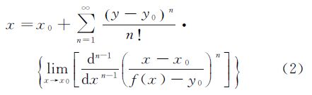
拉格朗日反演定理表明,在一阶导数不等于零的情况下,解析函数的反函数也可展开为泰勒级数。
2.2 基本思路
旋转椭球下,大地坐标(L,B,H)与空间直角坐标(X,Y,Z)之间的关系为
式中,
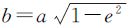
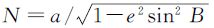 为卯酉圈曲率半径;a、e2分别为椭球的长半径和第一偏心率。
令 ,引入归化纬度μ,如图 1所示,则点P在大地经度为L的子午圈平面上的坐标为(W,Z),其在椭球面上的投影P0点的坐标可表示为(acos μ,bsin μ),因此有
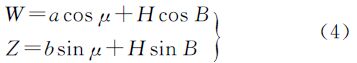
 ,归化纬度μ与大地纬度B的关系为
归化纬度μ与大地纬度B的关系一般记为
,归化纬度μ与大地纬度B的关系为
归化纬度μ与大地纬度B的关系一般记为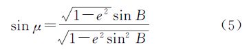
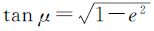 tan B,但其定义域不含B=90°,故本文采用式(5)。

|
| 图 1 空间直接坐标与大地坐标之关系 Fig. 1 Cartesian coordinates and geodetic coordinates |
图 1中,OI=Ne2sin B=be′2sin μ,OQ=Ne2cos B=ae2cos μ,C为P0点的曲率中心,坐标为(ae2cos3 μ,-be′2sin3 μ),对应的JK弧为椭圆的渐屈线。以P、C两点坐标求解tan B即为Bowring公式的思路。
由式(4)及图 1关系,可得
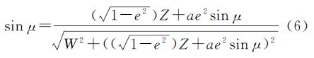
记s=sin μ,w=W/a,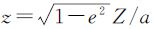 ,并构造函数
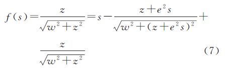
易得f(0)=0,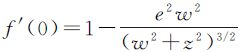 。则当(w2+z2)3/2≠e2w2时,f′(0)≠0,有
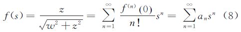
由拉格朗日反演定理,有
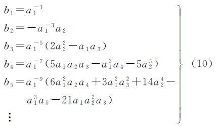
式(8)、式(9)两式中an、bn的关系为[25, 26]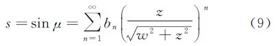
由归化纬度与大地纬度的关系式(5)可得

然后按式(12)求得大地高H

上式椭球面上及椭球外取“+”,椭球内取“-”。
3 系数求解及简化由上述讨论可首先求得式(8)的系数

再由关系式(10)可得

该系数较为复杂,为简化其结构,令
将其代入式(14),则有

综合以上各式可得

由此即可按式(11)、式(12)解得大地纬度B和大地高H。
以上为使推导过程方便,引入参数w、z,实际计算时,r、t1— t4可由空间直角坐标(X,Y,Z)直接得出
4 验算分析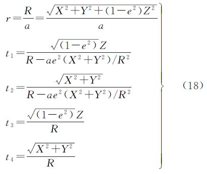
尽管式(17)本质上是以拉格朗日反演定理为基础的泰勒级数展开,但由于该问题的复杂性,按泰勒级数的余项理论给出其误差估计仍十分困难。为验证公式的正确性及其精度水平,下面以WGS-84椭球参数代入验算,并与经典的直接解法Bowring公式及迭代算法进行对比。
4.1 盲区对比式(17)与许多已有的其他解法一样,在接近椭球中心的区域存在盲区。
首先,由以上讨论可知,该解算方法要求(w2+z2)3/2-e2w2≠0。同时,经验算分析,当(w2+z2)3/2-e2w2<0、z≠0时,式(17)右端的值域超出sin μ的值域范围。由此可见,(w2+z2)3/2-e2w2≤0、z≠0所含区域为该方法的盲区。
已有算法的盲区(或多值区)多为椭球的渐屈线附近及其以内区域,如Bowring公式、经典迭代算法以及文献[20]所给的算法,与本文算法的盲区(w2+z2)3/2-e2w2≤0、z≠0,即
的区域关系如图 2所示。

|
| 图 2 盲区对比 Fig. 2 Comparison of the “dead zone” between Bowring’s formula and new method |
以上盲区范围距地心距离不超过42.84 km,处于地核内核内部,卫星大地测量一般不涉及这一区域。因此,从实用的角度看,各国学者一般最大范围取大地高-6×10⁶ ~+1010m的范围进行分析,本文亦取此范围进行分析。将本文算法与Bowring公式、经典迭代算法对比,其纬度解算误差对比如表 1和图 3所示。因高程解算精度主要取决于纬度解算,以下仅对纬度解算误差进行分析。
| 大地高/m | 最大纬度误差/(″) | ||||||
| Bowring公式 | 迭代算法 | 本文方法 | |||||
| 迭代3次 | 迭代4次 | 迭代5次 | 展开至b4项 | 展开至b5项 | |||
| -6×10⁶ | +54.38 | -7.42 | -7.41×10⁻¹ | -7.58×10⁻² | -3.03 | +3.80×10⁻¹ | |
| -4×10⁶ | +9.01×10⁻² | -4.76×10⁻³ | -7.59×10⁻⁵ | -1.24×10⁻⁶ | -2.09×10⁻⁴ | +3.91×10⁻⁶ | |
| -2×10⁶ | +3.58×10⁻³ | -4.15×10⁻⁴ | -3.59×10⁻⁶ | -3.18×10⁻⁸ | -9.71×10⁻⁶ | +9.67×10⁻⁸ | |
| -106 | +4.83×10⁻⁴ | -1.82×10⁻⁴ | -1.29×10⁻⁶ | -9.27×10⁻⁹ | -3.45×10⁻⁶ | +2.80×10⁻⁸ | |
| -104 | +2.90×10⁻⁸ | -9.27×10⁻⁵ | -5.52×10⁻⁷ | -3.36×10⁻⁹ | -1.47×10⁻⁶ | +1.01×10⁻⁸ | |
| -102 | +2.89×10⁻¹² | -9.22×10⁻⁵ | -5.47×10⁻⁷ | -3.33×10⁻⁹ | -1.46×10⁻⁶ | +1.00×10⁻⁸ | |
| 0 | 0.00 | -9.21×10⁻⁵ | -5.47×10⁻⁷ | -3.33×10⁻⁹ | -1.46×10⁻⁶ | +1.00×10⁻⁸ | |
| +102 | +2.89×10⁻¹² | -9.21×10⁻⁵ | -5.47×10⁻⁷ | -3.33×10⁻⁹ | -1.46×10⁻⁶ | +1.00×10⁻⁸ | |
| +104 | +2.88×10⁻⁸ | -9.15×10⁻⁵ | -5.43×10⁻⁷ | -3.30×10⁻⁹ | -1.45×10⁻⁶ | +9.89×10⁻⁹ | |
| +106 | +1.87×10⁻⁴ | -5.15×10⁻⁵ | -2.64×10⁻⁷ | -1.39×10⁻⁹ | -7.03×10⁻⁷ | +4.16×10⁻⁹ | |
| 2a | +1.74×10⁻³ | -1.14×10⁻⁶ | -2.26×10⁻⁹ | -4.57×10⁻¹² | -5.92×10⁻⁹ | +1.34×10⁻¹¹ | |
| 20 200 000 | +1.62×10⁻³ | -3.06×10⁻⁷ | -4.36×10⁻¹⁰ | -6.37×10⁻¹³ | -1.14×10⁻⁹ | +1.87×10⁻¹² | |
| +108 | +6.20×10⁻⁴ | -1.19×10⁻⁹ | -4.24×10⁻¹³ | -1.55×10⁻¹⁶ | -1.11×10⁻¹² | +4.52×10⁻¹⁶ | |
| +1010 | +7.45×10⁻⁶ | -1.52×10⁻¹⁷ | -5.76×10⁻²³ | -2.24×10⁻²⁸ | -1.50×10⁻²² | +6.25×10⁻²⁸ | |
| 注:H=20 200 000 m为GPS卫星运行轨道高度。 | |||||||

|
| 图 3 本文算法与Bowring公式、迭代算法的误差对比 Fig. 3 Comparison of the errors of geodetic latitude between Bowring’s formula,iterative algorithm and our algorithm |
为对比3种算法的计算效率,笔者在同一台计算机上,用Mathematica软件以纬度1°、大地高108 m为步长,分别利用3种方法计算B∈[0°,90°],H∈[0,1010]范围内91×101个点的总CPU执行时间,进而得到单个离散点的平均CPU执行时间,计算结果对比如表 2所示。
| 方法 | Bowring公式 | 3次迭代 | 4次迭代 | 5次迭代 | 本文方法b4项 | 本文方法b5项 |
| 9191点总CPU时间/s | 19.484 | 85.031 | 275.328 | 2 103.484 | 125.594 | 219.719 |
| 单点平均CPU时间/ms | 2.120 | 9.252 | 29.956 | 228.864 | 13.665 | 23.906 |
通过以上对比分析可知:
(1) 新算法与两种经典算法在接近椭球中心区域均存在盲区,需进一步研究,但实际应用一般不涉及这一区域。
(2) 精度上,若按照对应的点位误差不超过0.1 mm的原则,Bowring公式的有效范围约为-105 m≤H≤+105 m,在H≥+105 m以外区域解算精度迅速下降,最弱精度位于H=2a、B=π/4处,约+1.84×10-3″,相当于经线方向的0.11 m的点位误差。
新解法展开至b4项、b5项,以及迭代法迭代4次、5次在H≥-2×10⁻⁶ m的区域范围能够满足要求,有效范围比Bowring公式大。
(3) 计算效率上,Bowring公式最高,迭代法计算效率明显低于新解法计算效率。
综上可知,在-105 m≤H≤+105 m的范围内,Bowring公式精度最优,计算效率上占有显著优势,对于地面上的定位与导航应用,Bowring公式占据优势。
但实际上导航卫星大都是中地球轨道卫星,卫星高度在107m级,如GPS、GLONASS、北斗等卫星导航系统的卫星高度分别约为20 200 km、19 100 km、21 500 km,此时Bowring公式精度明显较弱,如表 1所示。兼顾精度和效率,本文算法较之于Bowring公式和迭代算法有一定优势。
此外,与其他直接解法相比,本文算法不必进行复杂的讨论,公式相对简洁,可根据精度需要决定末项取舍。
5 结 论本文以拉格朗日反演理论为基础,得到空间直角坐标向大地坐标转换的泰勒级数展开新方法,是一种新的直接解法,且经验算分析表明其精度可靠,能够满足实际应用精度要求。新解法由式(17)、式(18)两式构成,与已有直接解法相比,公式相对简洁,无须复杂讨论,可根据精度需要决定末项取舍,可扩展性好。同时,该解法随大地高的增加精度提高显著,这对现代空间技术是十分有利的,如航天工程、探月工程等。该方法的缺点是接近椭球中心区域存在盲区,这亦是Bowring公式、经典迭代算法等解法的共同问题,需要进一步研究。
| [1] | CHEN Junyong. Direct Solution of Transforming Cartesian to Geodetic Coordinates[C]//Special Issue on Geodesy. Beijing: Surveying and Mapping Press,1979:67-72.(陈俊勇. 空间直角坐标与大地坐标换算的直接解法[C]//大地测量研究专辑. 北京:测绘出版社,1979:67-72.) |
| [2] | ZENG Qixiong. Closed Formula for Direct Solution of Geodetic Coordinates from Rectangular Space Coordinates[J]. Acta Geodaetica et Cartographica Sinica, 1981,10(2):83-95.(曾启雄. 空间直角坐标直接解算大地坐标的闭合公式[J]. 测绘学报,1981,10(2):83-95.) |
| [3] | DEAKIN R E, HUNTER M N. Geometric Geodesy: Part A[M].Melbourne:[s.n.], 2010:89-102. |
| [4] | KONG Xiangyuan, GUO Jiming, LIU Zongquan. Foundation of Geodesy[M]. Wuhan: Wuhan University Press, 2001: 36-39.(孔祥元,郭际明,刘宗泉. 大地测量学基础[M]. 武汉:武汉大学出版社,2001:36-39.) |
| [5] | ZENG Qixiong. Direct Calculation Formula of Gauss Plane Rectangular Coordinates from Space Rectangular Coordinates[J]. Acta Geodaetica et Cartographica Sinica, 1993,22(1):74-79.(曾启雄. 空间直角坐标直接计算高斯平面直角坐标公式[J]. 测绘学报,1993,22(1):74-79.) |
| [6] | LIU Jingnan, LIU Dajie. The Influence of the Accuracy in Geodetic and Geocentric Coordinates on the Accuracy in the Results of Simultaneous Adjustment[J]. Acta Geodaetica et Cartographica Sinica, 1985,14(2):133-144.(刘经南,刘大杰.大地坐标和地心坐标精度对联合平差的精度影响[J]. 测绘学报,1985,14(2):133-144.) |
| [7] | LIU Dajie, BAI Zhengdong. A Mathematic Model of the 3-dimensional Adjustment of GPS Network[J]. Acta Geodaetica et Cartographica Sinica, 1997,26(1):37-41.(刘大杰,白征东. 一种GPS网三维平差的数学模型[J]. 测绘学报,1997,26(1):37-41.) |
| [8] | BOWRING B R. Transformation from Spatial to Geographical Coordinates[J]. Survey Review, 1976, 181: 323-327. |
| [9] | LIN K C, WANG J.Transformation from Geocentric to Geodetic Coordinates Using Newton’s Iteration[J]. Bulletin Géodésique, 1995, 69: 300-303. |
| [10] | FUKUSHIMA T. Fast Transform from Geocentric to Geodetic Coordinates[J]. Journal of Geodesy, 1999, 73: 603-610. |
| [11] | POLLARD J. Iterative Vector Methods for Computing Geodetic Latitude and Height from Rectangular Coordinates[J]. Journal of Geodesy, 2002, 76: 36-40. |
| [12] | FELTENS J. Vector Method to Compute the Cartesian (X,Y,Z) to Geodetic (φ,λ,h) Transformation on a Triaxial Ellipsoid[J]. Journal of Geodesy, 2009, 83: 129-137. |
| [13] | SHU Chanfang, LI Fei, SHEN Fei. A New Algorithm for Transforming from Cartesian to Geodetic Coordinates[J]. Geomatics and Information Science of Wuhan University, 2009,34(5):561-563.(束蝉方,李斐,沈飞. 空间直角坐标向大地坐标转换的新算法[J]. 武汉大学学报:信息科学版,2009,34(5):561-563.) |
| [14] | BORKOWSKI K M. Accurate Algorithms to Transform Geocentric to Geodetic Coordinates[J]. Bulletin Géodésique, 1989, 63: 50-56. |
| [15] | VERMEILLE H. Direct Transformation from Geocentric to Geodetic Coordinates[J]. Journal of Geodesy, 2002, 76: 451-454. |
| [16] | VERMEILLE H. Computing Geodetic Coordinates from Geocentric Coordinates[J]. Journal of Geodesy, 2004, 78: 94-95. |
| [17] | VERMEILLE H. An Analytical Method to Transform Geocentric into Geodetic Coordinates[J]. Journal of Geodesy, 2011, 85: 105-117. |
| [18] | FEATHERSTONE W E, CLAESSENS S J. Closed-form Transformation between Geodetic and Ellipsoidal Coordinates[J]. Studia Geophysica et Geodaetica, 2008, 52: 1-18. |
| [19] | TURNER J D. A Non-iterative and Non-singular Perturbation Solution for Transforming Cartesian to Geodetic Coordinates[J]. Journal of Geodesy, 2009, 83: 139-145. |
| [20] | ZHANG C D, HSU H T, WU X P. An Alternative Algebraic Algorithm to Transform Cartesian to Geodetic Coordinates[J]. Journal of Geodesy, 2005, 79: 413-420. |
| [21] | LIGAS M. Cartesian to Geodetic Coordinates Conversion on a Triaxial Ellipsoid[J]. Journal of Geodesy, 2012, 86: 249-256. |
| [22] | LAUREANO G V, IRENE P B. A Symbolic Analysis of Vermeille and Borkowski Polynomials for Transforming 3D Cartesian to Geodetic Coordinates[J]. Journal of Geodesy, 2009, 83: 1071-1081. |
| [23] | FUKUSHIMA T. Transformation from Cartesian to Geodetic Coordinates Accelerated by Halley’s Method[J]. Journal of Geodesy, 2006, 79: 689-693. |
| [24] | ABRAMOWITZ M, STEGUN I A. Handbook of Mathematical Functions with Formulas, Graphs, and Mathematical Tables[M].New York:Dover Publications Incorporation, 1972: 14-16. |
| [25] | WEISSTEIN E W.“Series Reversion” from Math World:A Wolfram Web Resource.[EB/OL].[2013-07-07].http://mathworld.wolfram.com/seriesreversion.html. |
| [26] | SLOANE N J A.The On-line Encyclopedia of Integer Sequences: The OEIS Foundation.[EB/OL].[2013-07-07]. http://oeis.org/. |