


2. 中国农业科学院农业资源与区域规划研究所农业部农业信息技术重点实验室, 北京 100081
2. Key Laboratory of Agri-informatics, Ministry of Agriculture, Institute of Agricultural Resources and Regional Planning, Chinese Academy of Agricultural Sciences, Beijing 100081, China
Electromagnetic wave scattering from a randomly rough surface requires complex mathematical treatment,but is of palpable importance in many fields of disciplines and bears itself in various applications spanned from surface treatment to remote sensing of terrain and sea [1, 2, 3, 4, 5, 6]. For example,it has been a common practice to retrieve,by analyzing the sensitivity of the scattering behavior and mechanisms,the geophysical parameters of interest from the scattering and/or emission measurements. Another example is that by knowing the scattering patterns,one may be able to detect the presence of the undesired random roughness of a reflective surface such as antenna reflector,and thus accordingly devise a means to correct or compensate the phase errors. Therefore,it has been both theoretically and practically motivated to study the electromagnetic wave scattering from the randomly rough surfaces. Research and progress,being a long historical track,of this topic have been well documented and still been keeping updates.
In order to tackle the complex and sometimes intricate mathematical derivations,while to remain a high level of accuracy beyond conventional models as well,notably,Kirchhoff and small perturbation method (SPM),the integral equation model (IEM) has been developed by Fung,et al.[3, 6, 7, 8] under few physical-justified assumptions. Driven by the need of predicting bistatic scattering and microwave emissivity,considerable efforts have been devoted to further improving the IEM accuracy [9, 10, 11, 12, 13, 14, 15, 16, 17, 18, 19] by removing some of the assumptions that imposed for the purpose of mathematical simplicity during the course of derivation. Another step leaping forward was the introduction of a transition function into the Fresnel reflection coefficients to take spatial dependences into account,removing the restrictions on the limits of surface roughness and permittivity [3, 11]. Though the approach is heuristic but self-consistent,it proves working perfectly for a broad range of surface dielectric and geometric parameters [6, 11, 14].
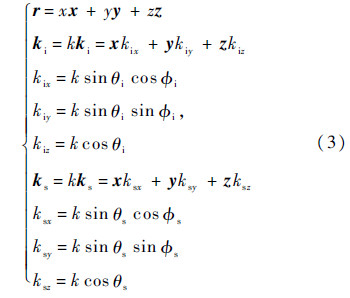
2 Formulation of wave scattering from a rough surface Referring to Fig. 1 with the direction of incidence (θi,φi) and scattering (θs,φs),suppose that a plane wave impinges onto a dielectric rough surface that scatters waves up into the incident plane and down into the lower medium,with the electric field Ei and magnetic field Hi being written as |
| Fig. 1 Geometry of bistatic scattering. |
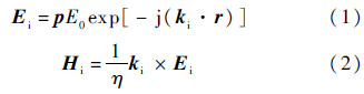
 ; p denotes the unit polarization vector,E0 the amplitude of the incident electric field Ei,η and ηt denote the intrinsic impedance of the upper and lower transmitted media,respectively. The position vector r,k-plane in incident direction ki and scattering direction ks are defined as follows,respectively
The polarization vector p is defined as hi and vi for incident linearly horizontal-polarized wave and vertical-polarized waves,respectively; and as hs and vs for scattering linearly horizontal-polarized wave and vertical-polarized waves,respectively.
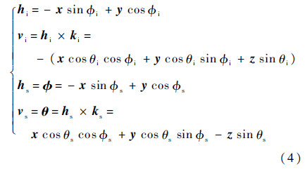
where φ and θ denote azimuthal and polar unit vectors,respectively.
The total electric field E(r) and magnetic field H(r) according to the Stratton-Chu formula could be expressed as [2, 5]
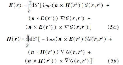

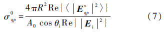
Once the scattered filed is solved,the scattering coefficient with q polarization is calculated as [2]
In view of Eq.(5),Ref. [5] states the Huygens’ principle.The field solution in a given volume V′ is completely determined by the tangential fields specified over the surface S′ enclosing V′. To find the surface fields,one has to solve the pair of Fredholm integral equations of 2nd kind. In our case,exact analytic solution is not possible. Approximate surface fields are estimated by iterative approach. The rough surface with irregular boundary is presented in Fig. 2,where  ,
, denote the upward re-radiation and downward re-radiation,going through upper medium and lower medium,respectively,θt denotes transmission angle,η0 wave impedance in air,ε0 permittivity in air,ηt wave impedance in lower medium,εt permittivity in lower medium,v vertical unit vector and d tangential unit vector normal to surface contour.
The completely analytic solution of rough surface is almost prohibitive. Instead,we seek the approximate estimate of the surface tangential fields by taking vector product with the unit surface normal on both sides of Eq. (6a),Eq.(6b) and,after reformulations [21],allowing an iterative scheme to find the estimates.
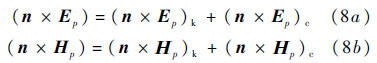
In IEM modelling [3, 7],the tangential surface fields is the sum of the Kirchhoff field and the complementary field,which are
where the Kirchhoff fields can be expressed as
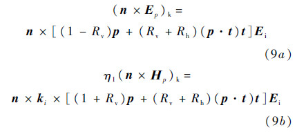
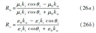
where Ep denotes electric field for p polarization,Ηpmagnetic field for p polarization,p polarization unit vector,t tangential unit vector and is tangential to the edge of surface contour; η1 wave impedance in medium 1,Rh and Rv denote Fresnel reflection coefficients for horizontally and vertically polarized waves,respectively.
The complementary surface field,which corrects the Kirchhoff estimates,is given as
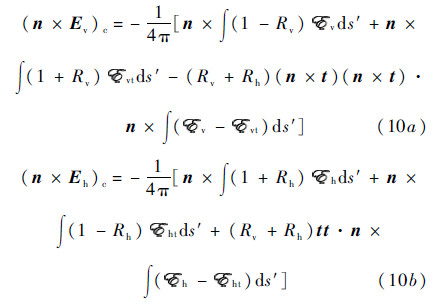
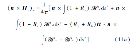
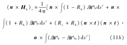
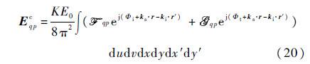
The electric and magnetic fields that appear inside the integrals above,
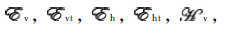
 and
and  are expressed as
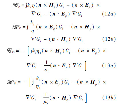
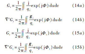
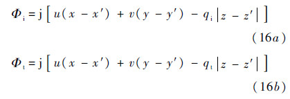
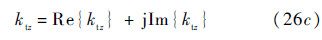
In Eq. (12) and Eq. (13),there involve Greens functions and theirs gradients in the upper and lower medium. To seek solutions by iterative scheme we make use of the spectral form,instead of spatial form,of the Green’s function [3, 7]

 . By substituting the Kirchhoff surface fields in Eq. (9a),Eq. (9b) into Eq. (12) and Eq. (13),we obtain the estimates of the complementary fields of Eq. (10) and Eq. (11). This may be seen as a 2nd iteration of seeking the solution of the integral equations governing the surface fields using Kirchhoff fields as the initial guess which is indeed a very good choice for fast convergence.
2.2 Far-zone scattered field
. By substituting the Kirchhoff surface fields in Eq. (9a),Eq. (9b) into Eq. (12) and Eq. (13),we obtain the estimates of the complementary fields of Eq. (10) and Eq. (11). This may be seen as a 2nd iteration of seeking the solution of the integral equations governing the surface fields using Kirchhoff fields as the initial guess which is indeed a very good choice for fast convergence.
2.2 Far-zone scattered field
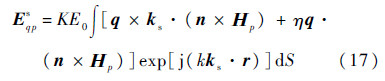
Now,with the surface tangential field estimates available,Esqp at far-zone distance R is readily calculated by making use of the Stratton-Chu formula.
 exp(-jkiR),E0 amplitude of the incident electric field.
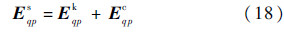
Corresponding to the Kirchhoff and the complementary surface fields in Eq. (8a),Eq. (8b),the far-zone scattered field may also be expressed as a sum of the Kirchhoff Ekqp and the complementary scattered fields Ecqp[3, 7]:

 and
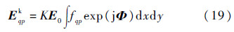
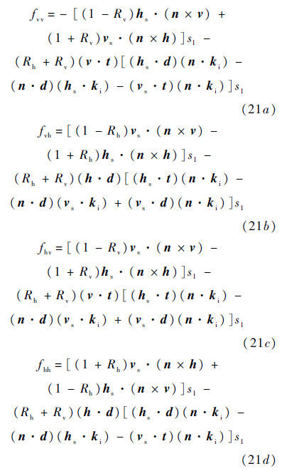
and  denote propagators. The Kirchhoff field coefficient fqp (both q and p denote h or v) appearing in Eq. (19)may be more explicitly written into the following form:
 ,zx and zy denote partial differential on x and y,respectively.
Noted that in IEM model,the terms involved (Rh+Rv) in Eq. (21) are all dropped off. Keeping in mind that the Kirchhoff field coefficient fqp is spatially dependent via the Fresnel reflection coefficients Rp(p denotes h or v) and the surface slope term s1. To make the integrals in Eq. (19) and Eq. (20) mathematically manageable in calculation of the average scattered power,we apply a stationary phase approximation while ignoring the edge diffraction,to obtain an estimate of the surface slopes. That is,the surface slopes are presumably independent of spatial variable,and are approximately determined by the directions of incident and scattering waves. To further tackle the mathematical manipulations,removal of the spatial dependence of the reflection coefficient will be made in Section 2.3. Keeping in mind that to what extent such estimate is valid or at least sufficiently accurate remains to be solved in further investigations.
Now go back to the complementary scattered field,which is much more complicated to deal with. Recalled that the complementary scattered field is contributed from the reradiated fields that may propagate through medium 1 and medium 2,in way of both upwardly and downwardly. The physical mechanism may be graphically represented by the field coefficients or the propagators, and ,as illustrated in Fig. 2. Further processing of the phase term involving the surface height,the propagators may be decomposed into the upward components designated by  and
and  and the downward components by
  and
and  ,mathematically appearing as the absolute terms in Eq. (16),physically denoting the change of propagation velocity in different media.
 |
| Fig. 2 Geometry of wave scattering and propagation from a rough surface |
In what follows,the complete phase terms are kept and all possible propagation waves are included. After straightforward but tedious mathematical manipulations,the complementary field coefficients can be obtained and put into compact forms for both the upward and downward propagations. Explicit expressions that are easy for numerical computation are given [14, 18]. For cross polarizations,we use an approximate reflection coefficient by taking the average of Rh and Rv: [3].
[3].
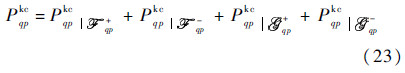
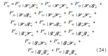
Now that with the scattered fields calculated,we perform ensemble averaging to compute the scattered power and the scattering coefficient. To gain more physical insights into the field interactions that produce the average power,the following expression for the incoherent average power Psqp is written as a sum of three terms: the Kirchhoff power Pkqp,the cross power Pkcqp due by the Kirchhoff field and the complementary,and the complementary power Pcqp.
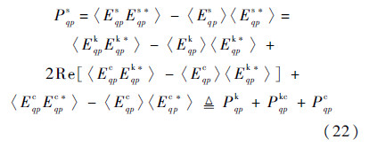
Geometrically,it is readily recognized that the cross power is the result of the interactions between the Kirchhoff field and the complementary field,being involved by four terms-two accounting for the upper medium propagation and the other two for the lower medium:
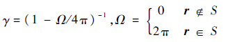
Now by substituting the Kirchhoff field and the complementary field into Eq. (24) and carrying out the ensemble averages,we may obtain an explicit expression of the incoherent average power. When the medium is very lossy,contributions from the lower medium propagation is expected to be small. In general,all modes must be included to get a more complete scattered power,as claimed in Ref.[19]. Whether it really so needs further investigation,however. After some algebraic manipulations and arrangements by Eq. (7) we can reach the final expression of a relatively compact form as
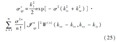
 denotes scattering amplitude; W(n)(ksx-kix,ksy-kiy) denotes the surface roughness spectrum of the surface related to the nth power of the surface correlation function by the two-dimensional Fourier transform,assuming that the surface height follows a Gaussian distribution.
Rh and Rv,are defined as follows,respectively:
denotes scattering amplitude; W(n)(ksx-kix,ksy-kiy) denotes the surface roughness spectrum of the surface related to the nth power of the surface correlation function by the two-dimensional Fourier transform,assuming that the surface height follows a Gaussian distribution.
Rh and Rv,are defined as follows,respectively:
After the above extensions,we shall name the IEM-based model as the AIEM model.
3 Comparison theoretical predictions with numerical simulations and experimental data 3.1 Comparison theoretical predictions with numerical simulationsThe prediction of scattering coefficient in scattering plane between the present model and numerical results of SSA (Small Slope Approximation) and MoM (Method of Moment) are shown in Fig. 3(a). The simulation data is adopted from Ref.[22] for a Gaussian correlated surface with εr=4-j1,kσ=0.5,kl=3.0 at incident angle of 30° and scattering angle between -60 o and 60°,where l denotes correlation length. Obviously,all the three predictions are quite close to each other except at larger backscattering angle. There is dip in specular direction shown by MoM and SSA,but not by AIEM. Doubling the surface roughness,results are given in Fig. 3(b) from which we can see that the angular trends by three predictions are similar to those in Fig. 3(a).
 |
| Fig. 3 Comparison of scattering coefficient between AIEM model and numerical results of MoM and SSA for both horizontal and vertical polarization for a Gaussian correlated surface with incident angle of 30° |
An excellent experimental data set for the purpose of comparison is adopted from Ref.[23] for a Gaussian correlated surface with σ=0.4cm,l=6cm; the scattering coefficient was measured at two incident angles,20° and 40°; incident frequencies of 2,5,and 10GHz,resulting in three different roughness scales but keeping at same surface slope as shown in Fig. 4. At this surface slope of Gaussian correlation,it is believed that the multiple scattering is very small. Fig. 4(a) shows the bistatic scattering behavior from which it is seen that both the AIEM and SPM agree well with the measured data except at scattering angles near 20° and beyond 20°. This might be due to a strong coherent contribution to the measurements,but still remains to be further confirmed. Measurements at frequency of 5GHz are presented in Fig. 4 (b). The surface is rougher for this case,so we plotted the GOM (Geometrical Optics Model) prediction as a reference. At this roughness scale with incident angle of 20°,neither GOM nor SPM matches with the experimental data,while the AIEM is in excellent agreement with the measured data. The scattering coefficient of HH and VV are closer compared to the measurement at 2GHz for higher frequency. Further increasing the incident angle to 40°,similar observations can be drawn,as is evident from Fig. 4(c). Also it is clear that along forward scattering near specular direction and beyond,the experimental data presented some degree of fluctuations-may be due to the remaining of coherent scattering which is stronger for smoother surface and tends to reduce as surface becomes rougher. At incident frequency of 10GHz,by closely inspecting Fig. 4(d) and Fig. 4 (e),both the AIEM and GOM present similar angular trends in forward scattering region and both agree well with the measured data. However,at backscattering with incident angle larger than 20°,the measurement reveals excessively higher than the model predictions of the AIEM and GOM. The difference seems not possibly be explained from the exclusion of multiple scattering,for the surface slope remains the same and small.
 |
| Fig. 4 Comparison of bistatic scattering coefficient between model predictions and measurement as function of scattering angle for a Gaussian correlated surface (σ=0.4cm, l=6cm) |
In bistatic scattering,it is of interest to observe the azimuthal pattern. From Fig. 1,if the transmitter is located at φi=0°,the null or dip of the scattering return presumably will occur near φs=90° for plane (flat) surface. Things are much more complicated,however. In what follows,we present two numerical cases to exam the roughness effect on the bistatic scattering pattern. The incident and scattering angles were chosen as θi=20°,θs=40°,respectively,and the surface relative permittivity of εr=10+j0.05. Fig. 5 displays the scattering coefficients for both HH and VV polarizations,where Fig. 5(a) is the case of smooth surface with  ,while in Fig. 5(b) the roughness is doubled (
 ,l=λ),λ being the radar wavelength. For reference,results of SPM and GOM models are also plotted.
 |
| Fig. 5 Effect of surface roughness on dip location in azimuthal plane (θi=20°,θs=40°,εr=10+j0.05) |
In small roughness cases,we see that both AIEM and SPM are in agreement,as expected. For VV polarization,the dip occurs ahead of that of HH polarization. As surface gets rougher,AIEM follows closely with GOM,also as expected. The dip now moves forward for HH polarization,but moves backward for VV polarization. Together the preceding features suggest that the dip location,which is highly polarization dependent,is an effective indicator of surface roughness. It is profoundly found that unlike SPM and GOM,the AIEM model consistently traces the dip location in the sense of roughness and polarization dependence.
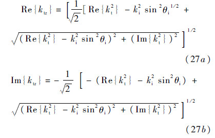
Fig. 6 displays the bistatic scattering coefficients of the SSA2 (Fig. 6(a)) and AIEM (Fig. 6(b)) in all four polarizations,VV,HH,HV,and VH [24] from a rough surface having rms height σ=λ/20,a Gaussian correlation function with correlation length l=λ/2 and a surface relative permittivity of εr=10+j0.05. Generally,similar behavior between SSA2 (second order small slope approximation) and AIEM,which are hemispherical patterns,is observed,including the locations of the dips that are dependent on the polarization [25].
5 Conclusions
Analysis of bistatic scattering from randomly rough surface was presented. The results can be summarized as follows.
1) Validation of the AIEM for bistatic scattering is made by comparison with numerical simulations and experimental measurements.
2) The AIEM model consistently traces the dip location in the sense of roughness and polarization dependence.
3) The hemispherical plots of AIEM,SSA2,MoM further confirm that the locations of the dips are dependent on the polarization.
4) Scattering in azimuthal plane is an effective indicator of surface roughness. The dependence of surface relative permittivity should be of importance and is under investigation.
5) The study of bistatic scattering through model simulations is useful for designing future radar measurement configuration as far as surface parameters retrieval is mattered.
| [1] | Beckman P,Spizzichino A.The scattering of electromagnetic waves from rough surfaces[M].Oxford:Pergamon Press,1963:215-285. |
| [2] | Ulaby F T,Moore R K,Fung A K.Microwave remote sensing:Active and passive,Vol.II-radar remote sensing and surface scattering and emission theory[M].Norwood,MA:Artech House,1982:922-1025. |
| [3] | Fung A K.Microwave scattering and emission models and their applications[M].Norwood,MA:Artech House,1994:1-10. |
| [4] | Voronovich A G.Wave scattering from rough surfaces[M].Berlin:Springer-Verlag,1994:1-5. |
| [5] | Tsang L,Kong J A.Scattering of electromagnetic waves:Advanced topics[M].New York:John Wiley & Sons,2001:65-118. |
| [6] | Fung A K,Chen K S,Microwave scattering and emission models for users[M].Norwood,MA:Artech House,2009:1-6. |
| [7] | Fung A K,Li Q,Chen K S.Backscattering from a randomly rough dielectric surface[J].IEEE Transactions on Geoscience and Remote Sensing,1992,30(2):356-369. |
| Click to display the text | |
| [8] | Chen K S,Fung A K,Weissman D E.A backscattering model for sea surfaces[J].IEEE Transactions on Geoscience and Remote Sensing,1992,30(4):811-817. |
| Click to display the text | |
| [9] | Hsieh C Y,Fung A K,Nesti G,et al.A further study of the IEM surface scattering model[J].IEEE Transactions on Geoscience and Remote Sensing,1997,35:901-909. |
| Click to display the text | |
| [10] | Chen K S,Wu T D,Tsay M K,et al.A note on the multiple scattering in an IEM model[J].IEEE Transactions on Geoscience and Remote Sensing,2000,38(1):249-256. |
| Click to display the text | |
| [11] | Wu T D,Chen K S,Shi J C,et al.A transition model for the reflection coefficient in surface scattering[J].IEEE Transactions on Geoscience and Remote Sensing,2001,39(9):2040-2050. |
| Click to display the text | |
| [12] | Álvarez-Pérez J L.An extension of the IEM/IEMM surface scattering model[J].Waves in Random Media,2001,11(3):307-329. |
| [13] | Fung A K,Liu W Y,Chen K S,et al.An improved IEM model for bistatic scattering[J].Journal of Electromagnetic Wave and Applications,2002,16(5):689-702. |
| Click to display the text | |
| [14] | Chen K S,Wu T D,Tsang L,et al.Emission of rough surfaces calculated by the integral eq.method with comparison to three-dimensional moment method simulations[J].IEEE Transactions on Geoscience and Remote Sensing,2003,41(1):90-101. |
| Click to display the text | |
| [15] | Wu T D,Chen K S.A reappraisal of the validity of the IEM model for backscattering from rough surfaces[J].IEEE Transactions on Geoscience and Remote Sensing,2004,42(8):743-753. |
| Click to display the text | |
| [16] | Fung A K,Chen K S.An update on IEM surface backscattering model[J].IEEE Geoscience and Remote Sensing Letters,2004,1(2):75-77. |
| Click to display the text | |
| [17] | Du Y.A new bistatic model for electromagnetic scattering from randomly rough surfaces[J].Waves Random Complex Media,2008,18(1):109-128. |
| Click to display the text | |
| [18] | Wu T D,Chen K S,Shi J C,et al.A study of AIEM model for bistatic scattering from randomly surfaces[J].IEEE Transactions on Geoscience and Remote Sensing,2008,46(9):2584-2598. |
| Click to display the text | |
| [19] | Álvarez-Pérez J L.The IEM2M rough-surface scattering model for complex-permittivity scattering media[J].Waves in Random and Complex Media,2012,22(2):207-233. |
| Click to display the text | |
| [20] | Poggio A J,Miller E K.Computer techniques for electromagnetics[M].Oxford:Pergamon Press,1973:159-260. |
| [21] | Li Z,Fung A K.A Reformulation of the surface field integral equation[J].Journal of Electromagnetic Waves and Application,1991,5:195-203. |
| Click to display the text | |
| [22] | Ewe H T,Johnson J T,Chen K S.A comparison study of the surface scattering models and numerical model[C]∥IEEE International Geoscience and Remote Sensing Symposium.Piscataway,NJ:IEEE Press,2001:2692-2694. |
| Click to display the text | |
| [23] | Macelloni G M,Nesti G,Pampaloni P,et al.Experimental validation of surface scattering and emission models[J].IEEE Transitions on Geoscience and Remote Sensing,2000,38(1):459-469. |
| Click to display the text | |
| [24] | Yardim C,Johnson J T,Burkholder R J,et al.An intercomparison of models for predicting bistatic scattering from rough surfaces[C]∥Proceedings of IGARSS.Piscataway,NJ:IEEE Press,2015,in press. |
| [25] | Johnson J T,Ouellette J D.Polarization features in bistatic scattering from rough surfaces[J].IEEE Transactions on Geoscience and Remote Sensing,2014,52(3):1616-1626. |
| Click to display the text |